Full infer Pipeline Examples
Source:vignettes/observed_stat_examples.Rmd
observed_stat_examples.RmdIntroduction
This vignette is intended to provide a set of examples that nearly
exhaustively demonstrate the functionalities provided by infer.
Commentary on these examples is limited—for more discussion of the
intuition behind the package, see the “Getting to Know infer” vignette,
accessible by calling vignette("infer").
Throughout this vignette, we’ll make use of the gss
dataset supplied by infer, which contains a sample of data from the
General Social Survey. See ?gss for more information on the
variables included and their source. Note that this data (and our
examples on it) are for demonstration purposes only, and will not
necessarily provide accurate estimates unless weighted properly. For
these examples, let’s suppose that this dataset is a representative
sample of a population we want to learn about: American adults. The data
looks like this:
## Rows: 500
## Columns: 11
## $ year    <dbl> 2014, 1994, 1998, 1996, 1994, 1996, 1990, 2016, 2000,…
## $ age     <dbl> 36, 34, 24, 42, 31, 32, 48, 36, 30, 33, 21, 30, 38, 4…
## $ sex     <fct> male, female, male, male, male, female, female, femal…
## $ college <fct> degree, no degree, degree, no degree, degree, no degr…
## $ partyid <fct> ind, rep, ind, ind, rep, rep, dem, ind, rep, dem, dem…
## $ hompop  <dbl> 3, 4, 1, 4, 2, 4, 2, 1, 5, 2, 4, 3, 4, 4, 2, 2, 3, 2,…
## $ hours   <dbl> 50, 31, 40, 40, 40, 53, 32, 20, 40, 40, 23, 52, 38, 7…
## $ income  <ord> $25000 or more, $20000 - 24999, $25000 or more, $2500…
## $ class   <fct> middle class, working class, working class, working c…
## $ finrela <fct> below average, below average, below average, above av…
## $ weight  <dbl> 0.8960, 1.0825, 0.5501, 1.0864, 1.0825, 1.0864, 1.062…
Hypothesis tests
One numerical variable (mean)
Calculating the observed statistic,
Alternatively, using the observe() wrapper to calculate
the observed statistic,
x_bar <- gss |>
  observe(response = hours, stat = "mean")
Then, generating the null distribution,
null_dist <- gss |>
  specify(response = hours) |>
  hypothesize(null = "point", mu = 40) |>
  generate(reps = 1000) |>
  calculate(stat = "mean")
Visualizing the observed statistic alongside the null distribution,
visualize(null_dist) +
  shade_p_value(obs_stat = x_bar, direction = "two-sided")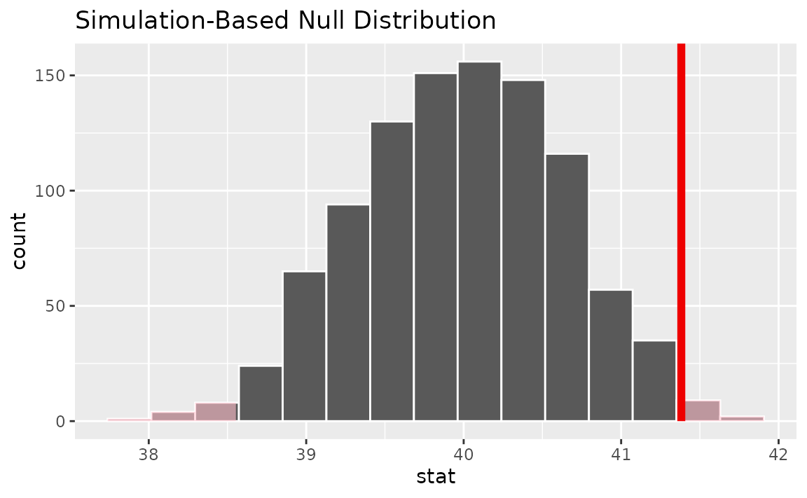
Calculating the p-value from the null distribution and observed statistic,
null_dist |>
  get_p_value(obs_stat = x_bar, direction = "two-sided")
## # A tibble: 1 × 1
## p_value
## <dbl>
## 1 0.022One numerical variable (standardized mean )
Calculating the observed statistic,
t_bar <- gss |>
  specify(response = hours) |>
  hypothesize(null = "point", mu = 40) |>
  calculate(stat = "t")
Alternatively, using the observe() wrapper to calculate
the observed statistic,
t_bar <- gss |>
  observe(response = hours, null = "point", mu = 40, stat = "t")
Then, generating the null distribution,
null_dist <- gss |>
  specify(response = hours) |>
  hypothesize(null = "point", mu = 40) |>
  generate(reps = 1000) |>
  calculate(stat = "t")
Alternatively, finding the null distribution using theoretical
methods using the assume() verb,
Visualizing the observed statistic alongside the null distribution,
visualize(null_dist) +
  shade_p_value(obs_stat = t_bar, direction = "two-sided")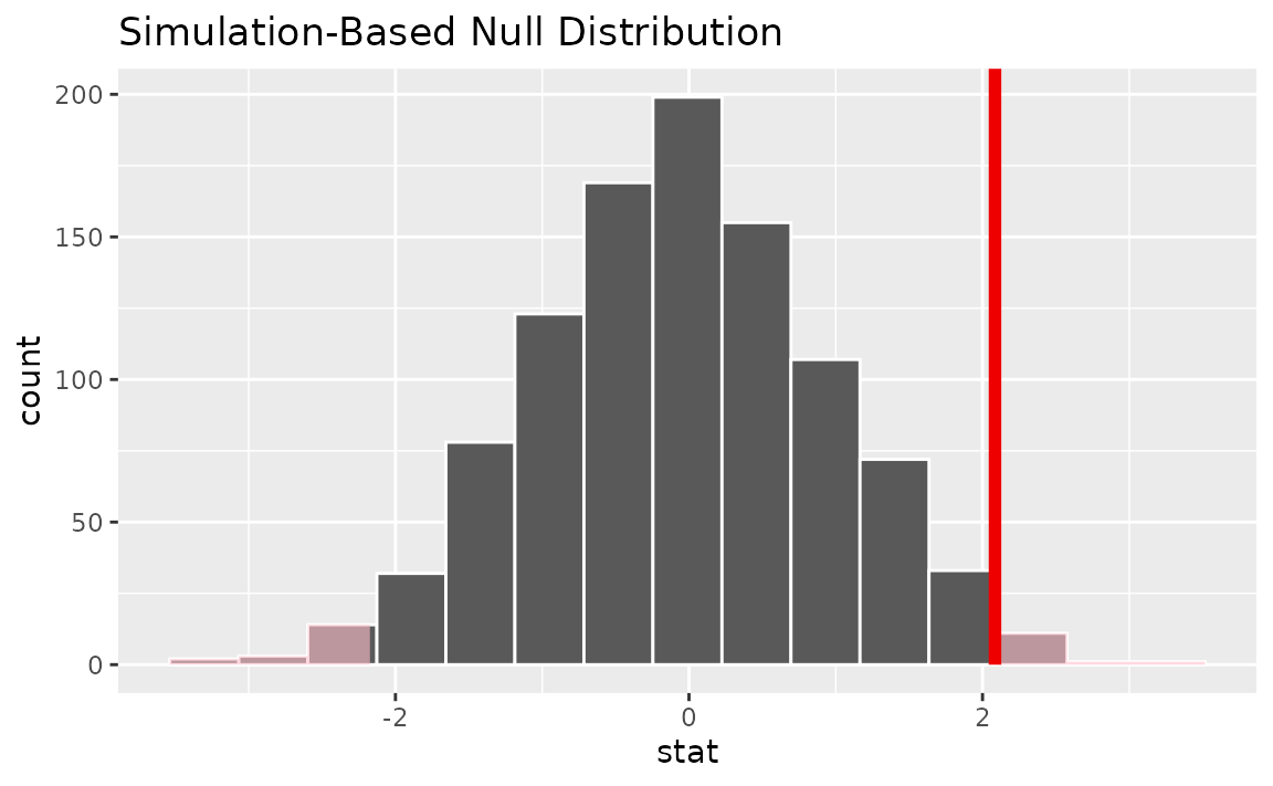
Alternatively, visualizing the observed statistic using the theory-based null distribution,
visualize(null_dist_theory) +
  shade_p_value(obs_stat = t_bar, direction = "two-sided")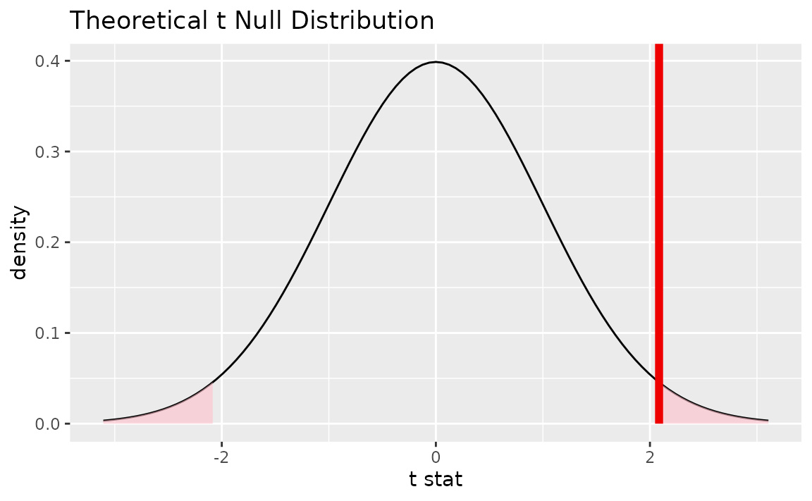
Alternatively, visualizing the observed statistic using both of the null distributions,
visualize(null_dist, method = "both") +
  shade_p_value(obs_stat = t_bar, direction = "two-sided")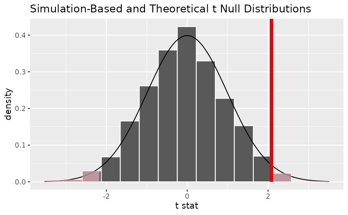
Note that the above code makes use of the randomization-based null distribution.
Calculating the p-value from the null distribution and observed statistic,
null_dist |>
  get_p_value(obs_stat = t_bar, direction = "two-sided")
## # A tibble: 1 × 1
## p_value
## <dbl>
## 1 0.028Alternatively, using the t_test() wrapper:
gss |>
  t_test(response = hours, mu = 40)
## # A tibble: 1 × 7
## statistic t_df p_value alternative estimate lower_ci upper_ci
## <dbl> <dbl> <dbl> <chr> <dbl> <dbl> <dbl>
## 1 2.09 499 0.0376 two.sided 41.4 40.1 42.7infer does not support testing on one numerical variable
via the z distribution.
One numerical variable (median)
Calculating the observed statistic,
Alternatively, using the observe() wrapper to calculate
the observed statistic,
x_tilde <- gss |>
  observe(response = age, stat = "median")
Then, generating the null distribution,
null_dist <- gss |>
  specify(response = age) |>
  hypothesize(null = "point", med = 40) |>
  generate(reps = 1000) |>
  calculate(stat = "median")
Visualizing the observed statistic alongside the null distribution,
visualize(null_dist) +
  shade_p_value(obs_stat = x_tilde, direction = "two-sided")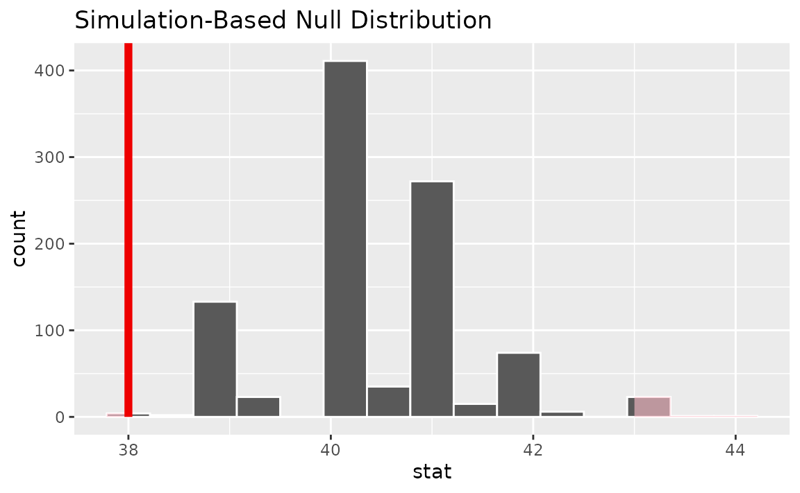
Calculating the p-value from the null distribution and observed statistic,
null_dist |>
  get_p_value(obs_stat = x_tilde, direction = "two-sided")
## # A tibble: 1 × 1
## p_value
## <dbl>
## 1 0.008One numerical variable (paired)
The example under this header is compatible with stats
"mean", "median", "sum", and
"sd".
Suppose that each of these survey respondents had provided the number
of hours worked per week when surveyed 5 years prior,
encoded as hours_previous.
set.seed(1)

gss_paired <- gss |>
   mutate(
      hours_previous = hours + 5 - rpois(nrow(gss), 4.8),
      diff = hours - hours_previous
   )

gss_paired |>
   select(hours, hours_previous, diff)
## # A tibble: 500 × 3
## hours hours_previous diff
## <dbl> <dbl> <dbl>
## 1 50 52 -2
## 2 31 32 -1
## 3 40 40 0
## 4 40 37 3
## 5 40 42 -2
## 6 53 50 3
## 7 32 28 4
## 8 20 19 1
## 9 40 40 0
## 10 40 43 -3
## # ℹ 490 more rowsWe’d like to test the null hypothesis that the "mean"
hours worked per week did not change between the sampled time and five
years prior.
infer supports paired hypothesis testing via the
null = "paired independence" argument to
hypothesize().
Calculating the observed statistic,
Alternatively, using the observe() wrapper to calculate
the observed statistic,
x_tilde <- gss_paired |>
  observe(response = diff, stat = "mean")
Then, generating the null distribution,
null_dist <- gss_paired |>
  specify(response = diff) |>
  hypothesize(null = "paired independence") |>
  generate(reps = 1000, type = "permute") |>
  calculate(stat = "mean")
Note that the diff column itself is not permuted, but
rather the signs of the values in the column.
Visualizing the observed statistic alongside the null distribution,
visualize(null_dist) +
  shade_p_value(obs_stat = x_tilde, direction = "two-sided")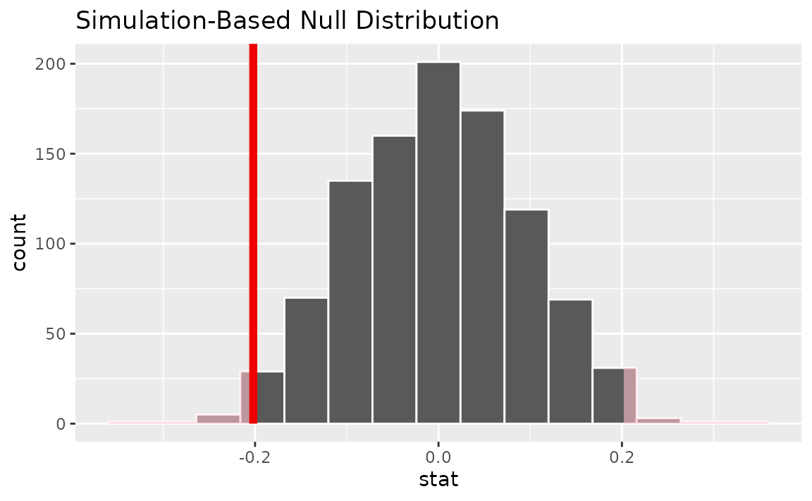
Calculating the p-value from the null distribution and observed statistic,
null_dist |>
  get_p_value(obs_stat = x_tilde, direction = "two-sided")
## # A tibble: 1 × 1
## p_value
## <dbl>
## 1 0.028One categorical (one proportion)
Calculating the observed statistic,
Alternatively, using the observe() wrapper to calculate
the observed statistic,
p_hat <- gss |>
  observe(response = sex, success = "female", stat = "prop")
Then, generating the null distribution,
null_dist <- gss |>
  specify(response = sex, success = "female") |>
  hypothesize(null = "point", p = .5) |>
  generate(reps = 1000) |>
  calculate(stat = "prop")
Visualizing the observed statistic alongside the null distribution,
visualize(null_dist) +
  shade_p_value(obs_stat = p_hat, direction = "two-sided")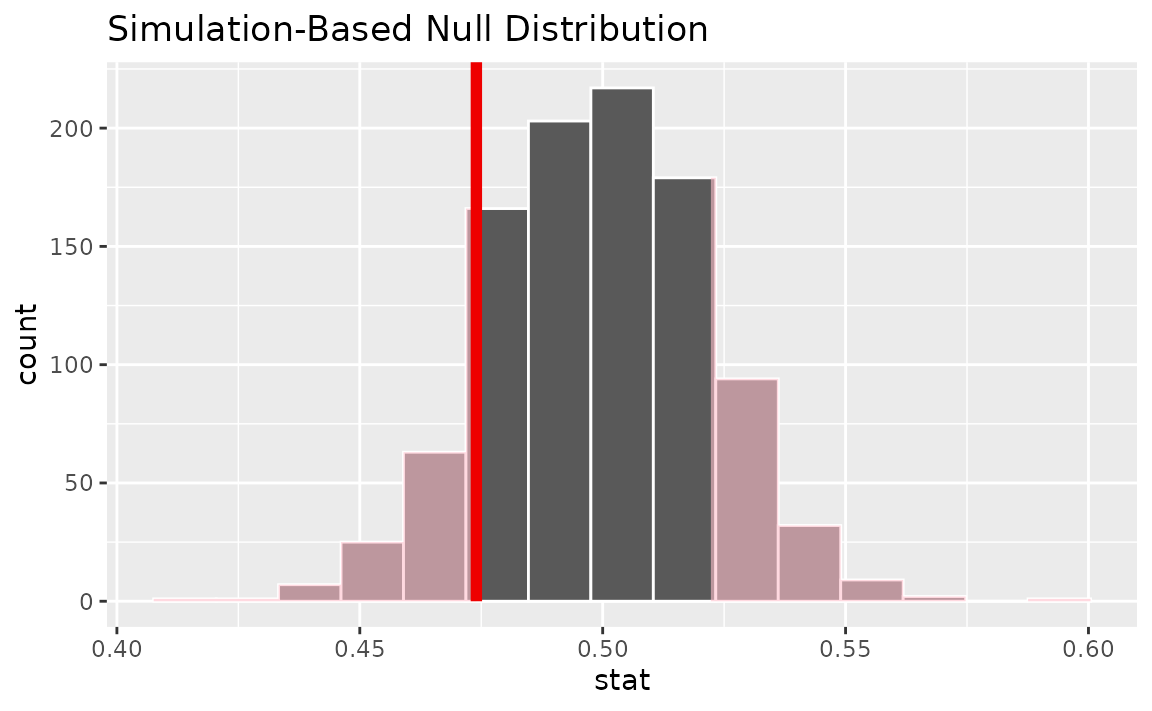
Calculating the p-value from the null distribution and observed statistic,
null_dist |>
  get_p_value(obs_stat = p_hat, direction = "two-sided")
## # A tibble: 1 × 1
## p_value
## <dbl>
## 1 0.276Note that logical variables will be coerced to factors:
null_dist <- gss |>
  dplyr::mutate(is_female = (sex == "female")) |>
  specify(response = is_female, success = "TRUE") |>
  hypothesize(null = "point", p = .5) |>
  generate(reps = 1000) |>
  calculate(stat = "prop")
One categorical variable (standardized proportion )
Calculating the observed statistic,
p_hat <- gss |>
  specify(response = sex, success = "female") |>
  hypothesize(null = "point", p = .5) |>
  calculate(stat = "z")
Alternatively, using the observe() wrapper to calculate
the observed statistic,
p_hat <- gss |>
  observe(response = sex, success = "female", null = "point", p = .5, stat = "z")
Then, generating the null distribution,
null_dist <- gss |>
  specify(response = sex, success = "female") |>
  hypothesize(null = "point", p = .5) |>
  generate(reps = 1000, type = "draw") |>
  calculate(stat = "z")
Visualizing the observed statistic alongside the null distribution,
visualize(null_dist) +
  shade_p_value(obs_stat = p_hat, direction = "two-sided")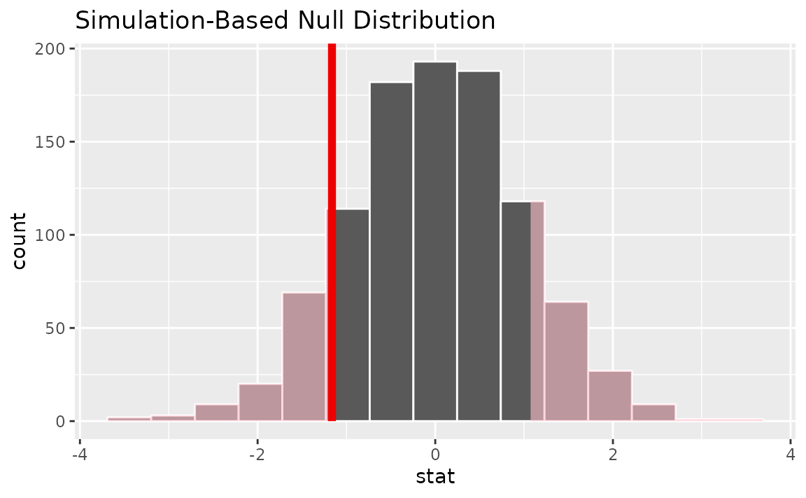
Calculating the p-value from the null distribution and observed statistic,
null_dist |>
  get_p_value(obs_stat = p_hat, direction = "two-sided")
## # A tibble: 1 × 1
## p_value
## <dbl>
## 1 0.252The package also supplies a wrapper around prop.test()
for tests of a single proportion on tidy data.
prop_test(gss,
          college ~ NULL,
          p = .2)
## # A tibble: 1 × 4
## statistic chisq_df p_value alternative
## <dbl> <int> <dbl> <chr>
## 1 636. 1 2.98e-140 two.sidedinfer does not support testing two means via the z
distribution.
Two categorical (2 level) variables
The infer package provides several statistics to work
with data of this type. One of them is the statistic for difference in
proportions.
Calculating the observed statistic,
d_hat <- gss |>
  specify(college ~ sex, success = "no degree") |>
  calculate(stat = "diff in props", order = c("female", "male"))
Alternatively, using the observe() wrapper to calculate
the observed statistic,
d_hat <- gss |>
  observe(
    college ~ sex,
    success = "no degree",
    stat = "diff in props", order = c("female", "male")
  )
Then, generating the null distribution,
null_dist <- gss |>
  specify(college ~ sex, success = "no degree") |>
  hypothesize(null = "independence") |>
  generate(reps = 1000) |>
  calculate(stat = "diff in props", order = c("female", "male"))
Visualizing the observed statistic alongside the null distribution,
visualize(null_dist) +
  shade_p_value(obs_stat = d_hat, direction = "two-sided")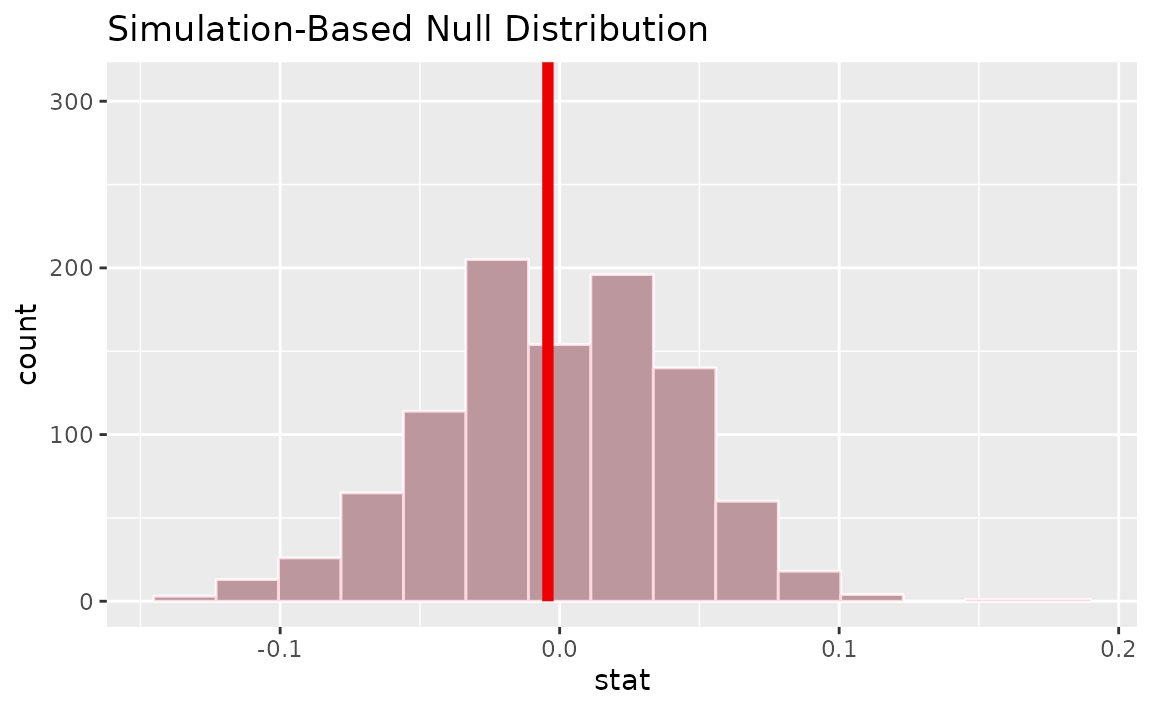
Calculating the p-value from the null distribution and observed statistic,
null_dist |>
  get_p_value(obs_stat = d_hat, direction = "two-sided")
## # A tibble: 1 × 1
## p_value
## <dbl>
## 1 1infer also provides functionality to calculate ratios of proportions.
The workflow looks similar to that for diff in props.
Calculating the observed statistic,
r_hat <- gss |>
  specify(college ~ sex, success = "no degree") |>
  calculate(stat = "ratio of props", order = c("female", "male"))
Alternatively, using the observe() wrapper to calculate
the observed statistic,
r_hat <- gss |>
  observe(college ~ sex, success = "no degree",
          stat = "ratio of props", order = c("female", "male"))
Then, generating the null distribution,
null_dist <- gss |>
  specify(college ~ sex, success = "no degree") |>
  hypothesize(null = "independence") |>
  generate(reps = 1000) |>
  calculate(stat = "ratio of props", order = c("female", "male"))
Visualizing the observed statistic alongside the null distribution,
visualize(null_dist) +
  shade_p_value(obs_stat = r_hat, direction = "two-sided")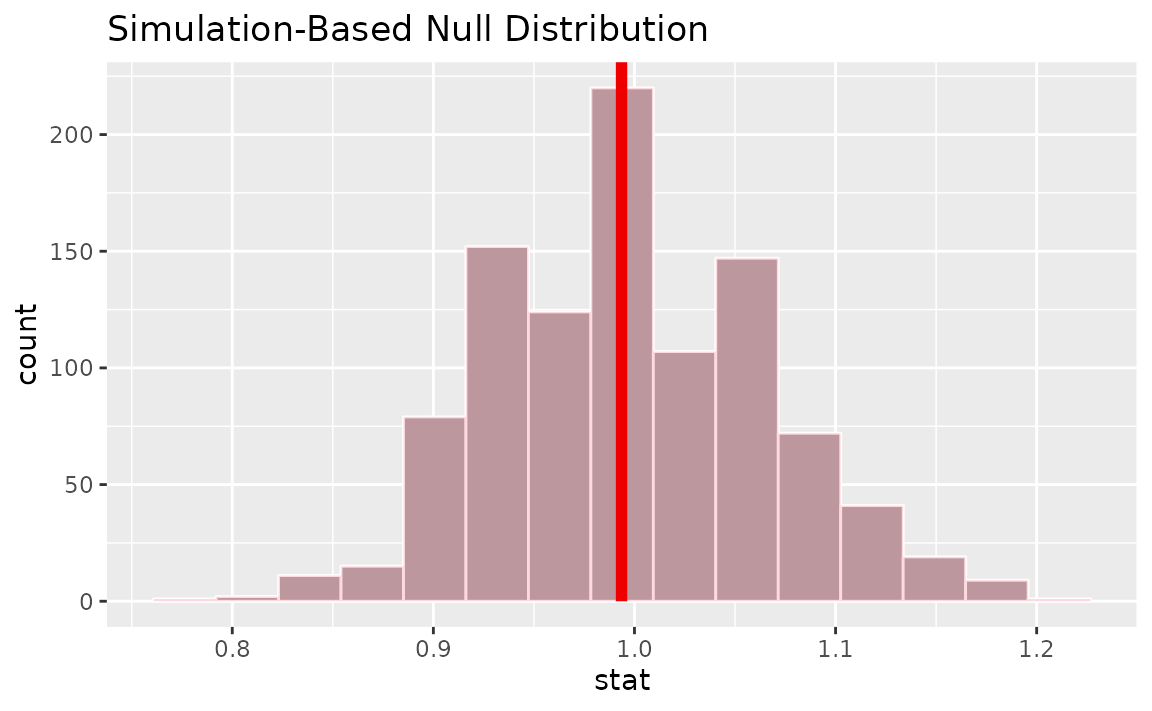
Calculating the p-value from the null distribution and observed statistic,
null_dist |>
  get_p_value(obs_stat = r_hat, direction = "two-sided")
## # A tibble: 1 × 1
## p_value
## <dbl>
## 1 1In addition, the package provides functionality to calculate odds
ratios. The workflow also looks similar to that for
diff in props.
Calculating the observed statistic,
or_hat <- gss |>
  specify(college ~ sex, success = "no degree") |>
  calculate(stat = "odds ratio", order = c("female", "male"))
Then, generating the null distribution,
null_dist <- gss |>
  specify(college ~ sex, success = "no degree") |>
  hypothesize(null = "independence") |>
  generate(reps = 1000) |>
  calculate(stat = "odds ratio", order = c("female", "male"))
Visualizing the observed statistic alongside the null distribution,
visualize(null_dist) +
  shade_p_value(obs_stat = or_hat, direction = "two-sided")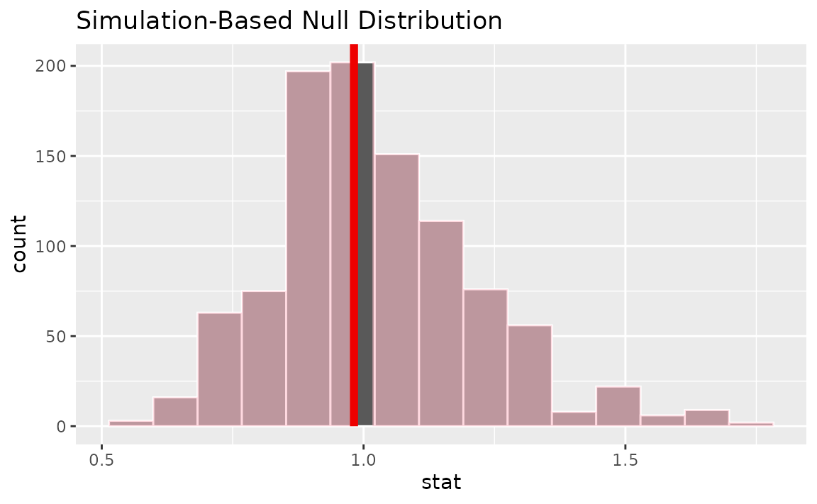
Calculating the p-value from the null distribution and observed statistic,
null_dist |>
  get_p_value(obs_stat = or_hat, direction = "two-sided")
## # A tibble: 1 × 1
## p_value
## <dbl>
## 1 0.984Two categorical (2 level) variables (z)
Finding the standardized observed statistic,
z_hat <- gss |>
  specify(college ~ sex, success = "no degree") |>
  hypothesize(null = "independence") |>
  calculate(stat = "z", order = c("female", "male"))
Alternatively, using the observe() wrapper to calculate
the observed statistic,
z_hat <- gss |>
  observe(college ~ sex, success = "no degree",
          stat = "z", order = c("female", "male"))
Then, generating the null distribution,
null_dist <- gss |>
  specify(college ~ sex, success = "no degree") |>
  hypothesize(null = "independence") |>
  generate(reps = 1000) |>
  calculate(stat = "z", order = c("female", "male"))
Alternatively, finding the null distribution using theoretical
methods using the assume() verb,
Visualizing the observed statistic alongside the null distribution,
visualize(null_dist) +
  shade_p_value(obs_stat = z_hat, direction = "two-sided")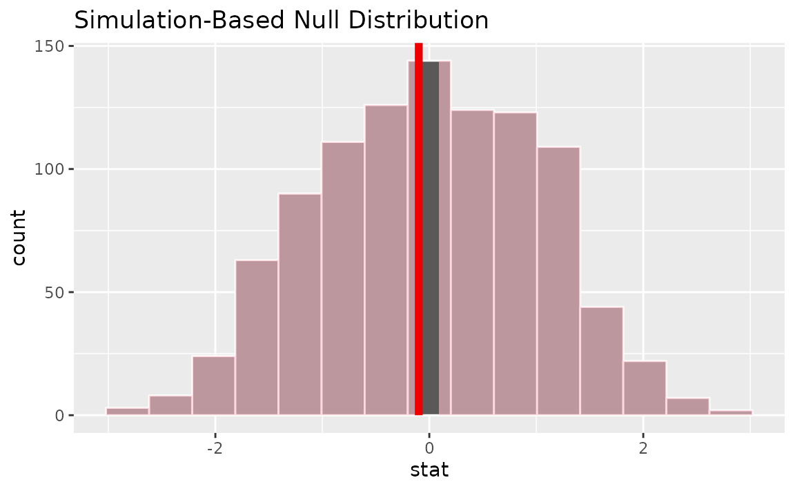
Alternatively, visualizing the observed statistic using the theory-based null distribution,
visualize(null_dist_theory) +
  shade_p_value(obs_stat = z_hat, direction = "two-sided")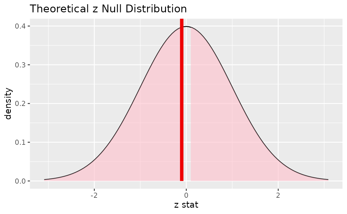
Alternatively, visualizing the observed statistic using both of the null distributions,
visualize(null_dist, method = "both") +
  shade_p_value(obs_stat = z_hat, direction = "two-sided")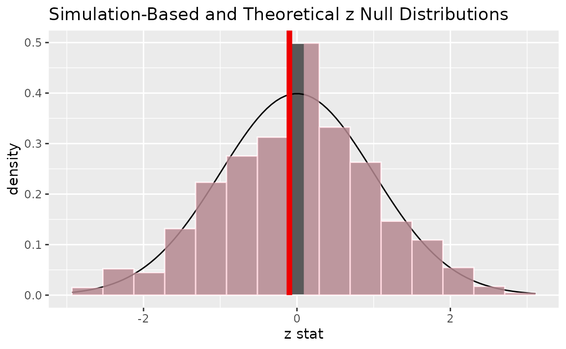
Note that the above code makes use of the randomization-based null distribution.
Calculating the p-value from the null distribution and observed statistic,
null_dist |>
  get_p_value(obs_stat = z_hat, direction = "two-sided")
## # A tibble: 1 × 1
## p_value
## <dbl>
## 1 0.98Note the similarities in this plot and the previous one.
The package also supplies a wrapper around prop.test to
allow for tests of equality of proportions on tidy data.
## # A tibble: 1 × 6
##   statistic chisq_df p_value alternative lower_ci upper_ci
##       <dbl>    <dbl>   <dbl> <chr>          <dbl>    <dbl>
## 1 0.0000204        1   0.996 two.sided    -0.0918   0.0834
One categorical (>2 level) - GoF
Calculating the observed statistic,
Note the need to add in the hypothesized values here to compute the observed statistic.
Chisq_hat <- gss |>
  specify(response = finrela) |>
  hypothesize(
    null = "point",
    p = c(
      "far below average" = 1 / 6,
      "below average" = 1 / 6,
      "average" = 1 / 6,
      "above average" = 1 / 6,
      "far above average" = 1 / 6,
      "DK" = 1 / 6
    )
  ) |>
  calculate(stat = "Chisq")
Alternatively, using the observe() wrapper to calculate
the observed statistic,
Chisq_hat <- gss |>
  observe(
    response = finrela,
    null = "point",
    p = c(
      "far below average" = 1 / 6,
      "below average" = 1 / 6,
      "average" = 1 / 6,
      "above average" = 1 / 6,
      "far above average" = 1 / 6,
      "DK" = 1 / 6
    ),
    stat = "Chisq"
  )
Then, generating the null distribution,
null_dist <- gss |>
  specify(response = finrela) |>
  hypothesize(
    null = "point",
    p = c(
      "far below average" = 1 / 6,
      "below average" = 1 / 6,
      "average" = 1 / 6,
      "above average" = 1 / 6,
      "far above average" = 1 / 6,
      "DK" = 1 / 6
    )
  ) |>
  generate(reps = 1000, type = "draw") |>
  calculate(stat = "Chisq")
Alternatively, finding the null distribution using theoretical
methods using the assume() verb,
Visualizing the observed statistic alongside the null distribution,
visualize(null_dist) +
  shade_p_value(obs_stat = Chisq_hat, direction = "greater")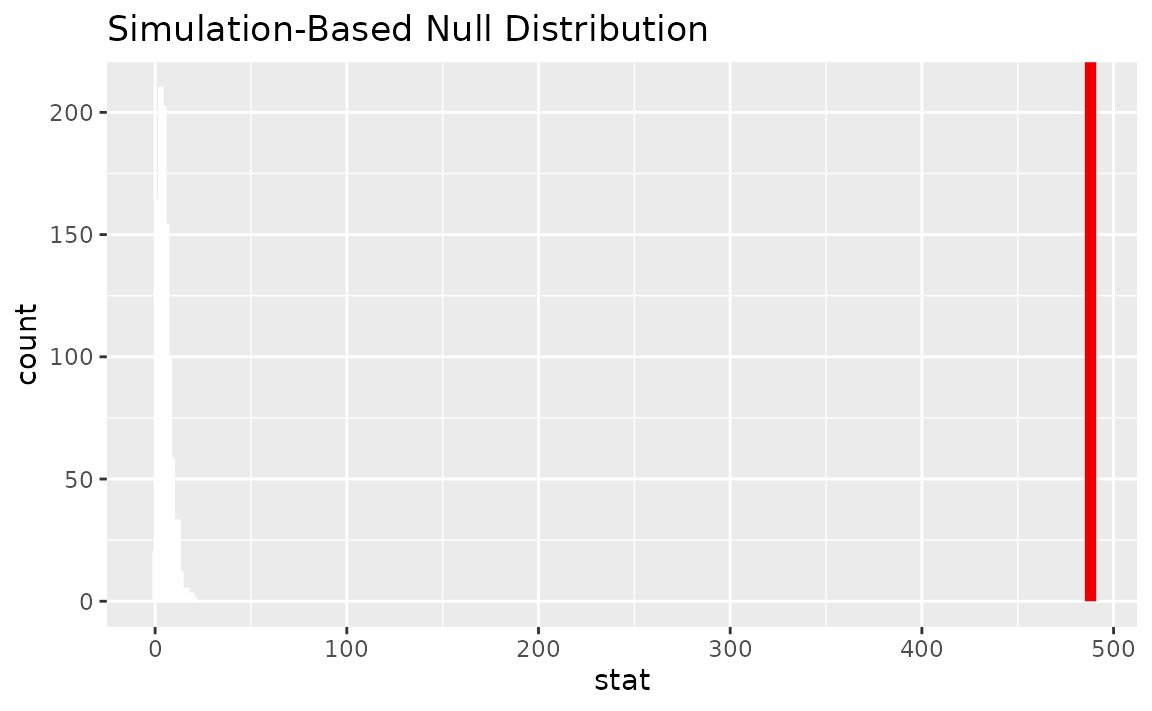
Alternatively, visualizing the observed statistic using the theory-based null distribution,
visualize(null_dist_theory) +
  shade_p_value(obs_stat = Chisq_hat, direction = "greater")
Alternatively, visualizing the observed statistic using both of the null distributions,
visualize(null_dist_theory, method = "both") +
  shade_p_value(obs_stat = Chisq_hat, direction = "greater")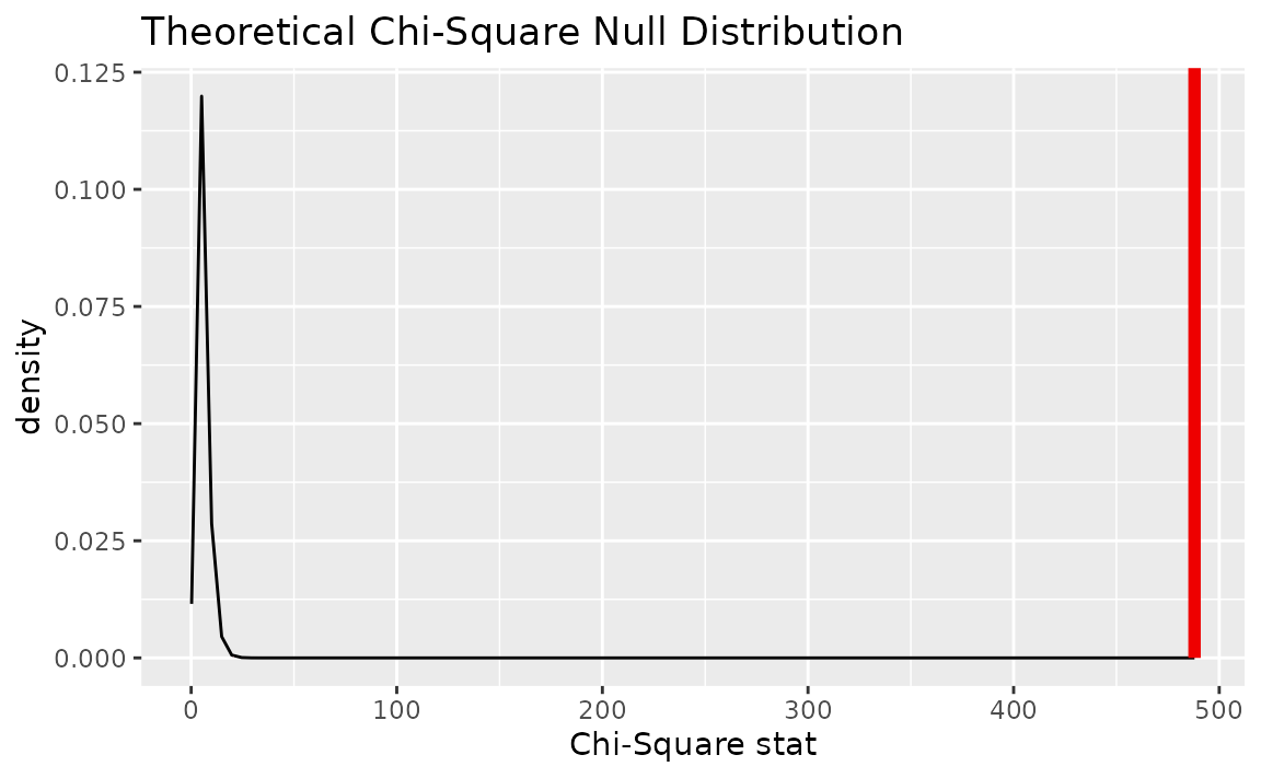
Note that the above code makes use of the randomization-based null distribution.
Calculating the p-value from the null distribution and observed statistic,
null_dist |>
  get_p_value(obs_stat = Chisq_hat, direction = "greater")
## # A tibble: 1 × 1
## p_value
## <dbl>
## 1 0Alternatively, using the chisq_test wrapper:
chisq_test(
  gss,
  response = finrela,
  p = c(
    "far below average" = 1 / 6,
    "below average" = 1 / 6,
    "average" = 1 / 6,
    "above average" = 1 / 6,
    "far above average" = 1 / 6,
    "DK" = 1 / 6
  )
)
## # A tibble: 1 × 3
## statistic chisq_df p_value
## <dbl> <dbl> <dbl>
## 1 488. 5 3.13e-103Two categorical (>2 level): Chi-squared test of independence
Calculating the observed statistic,
Chisq_hat <- gss |>
  specify(formula = finrela ~ sex) |>
  hypothesize(null = "independence") |>
  calculate(stat = "Chisq")
Alternatively, using the observe() wrapper to calculate
the observed statistic,
Chisq_hat <- gss |>
  observe(formula = finrela ~ sex, stat = "Chisq")
Then, generating the null distribution,
null_dist <- gss |>
  specify(finrela ~ sex) |>
  hypothesize(null = "independence") |>
  generate(reps = 1000, type = "permute") |>
  calculate(stat = "Chisq")
Alternatively, finding the null distribution using theoretical
methods using the assume() verb,
Visualizing the observed statistic alongside the null distribution,
visualize(null_dist) +
  shade_p_value(obs_stat = Chisq_hat, direction = "greater")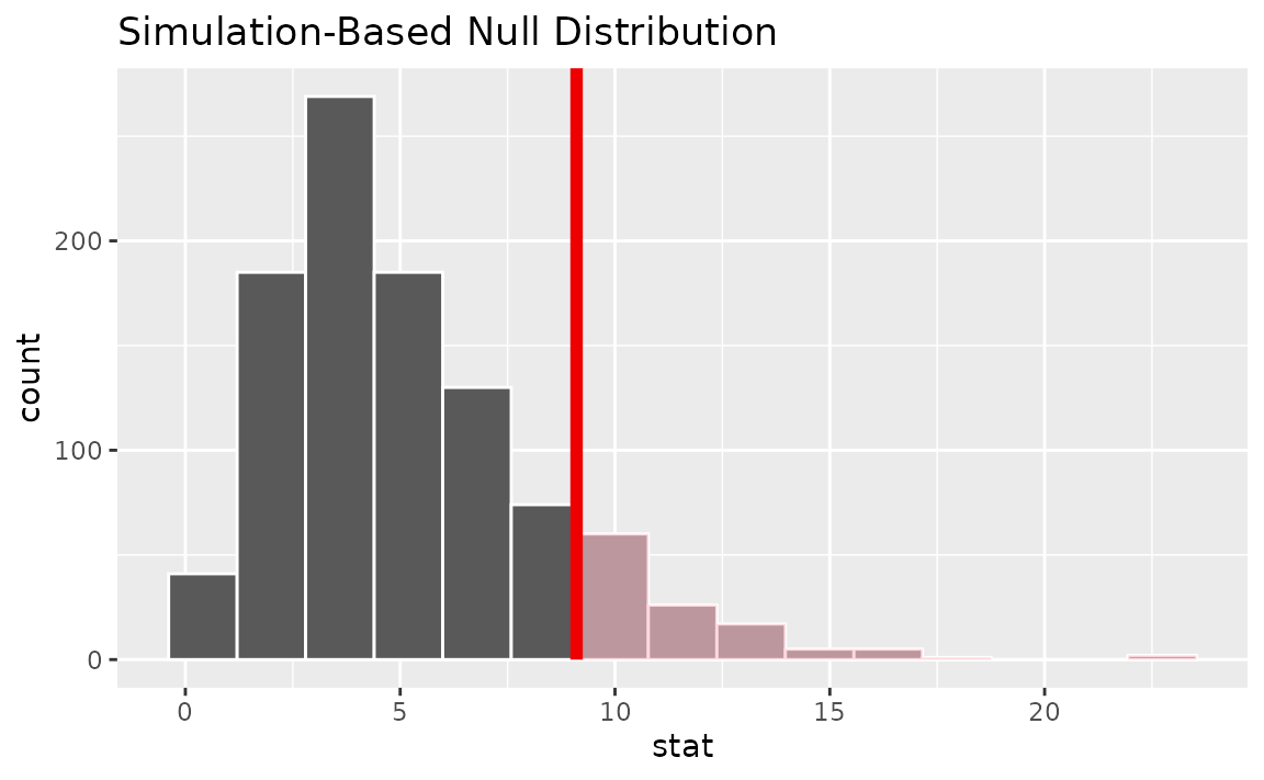
Alternatively, visualizing the observed statistic using the theory-based null distribution,
visualize(null_dist_theory) +
  shade_p_value(obs_stat = Chisq_hat, direction = "greater")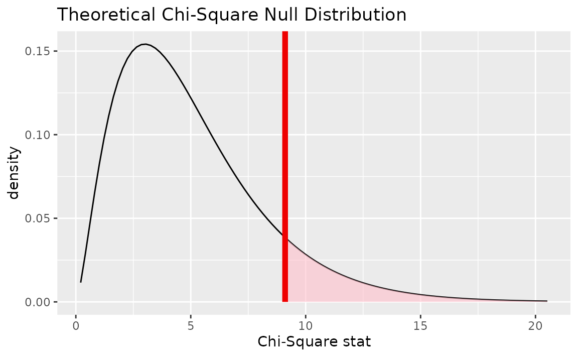
Alternatively, visualizing the observed statistic using both of the null distributions,
visualize(null_dist, method = "both") +
  shade_p_value(obs_stat = Chisq_hat, direction = "greater")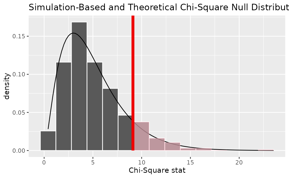
Note that the above code makes use of the randomization-based null distribution.
Calculating the p-value from the null distribution and observed statistic,
null_dist |>
  get_p_value(obs_stat = Chisq_hat, direction = "greater")
## # A tibble: 1 × 1
## p_value
## <dbl>
## 1 0.118Alternatively, using the wrapper to carry out the test,
gss |>
  chisq_test(formula = finrela ~ sex)
## # A tibble: 1 × 3
## statistic chisq_df p_value
## <dbl> <int> <dbl>
## 1 9.11 5 0.105One numerical variable, one categorical (2 levels) (diff in means)
Calculating the observed statistic,
d_hat <- gss |>
  specify(age ~ college) |>
  calculate(stat = "diff in means", order = c("degree", "no degree"))
Alternatively, using the observe() wrapper to calculate
the observed statistic,
Then, generating the null distribution,
null_dist <- gss |>
  specify(age ~ college) |>
  hypothesize(null = "independence") |>
  generate(reps = 1000, type = "permute") |>
  calculate(stat = "diff in means", order = c("degree", "no degree"))
Visualizing the observed statistic alongside the null distribution,
visualize(null_dist) +
  shade_p_value(obs_stat = d_hat, direction = "two-sided")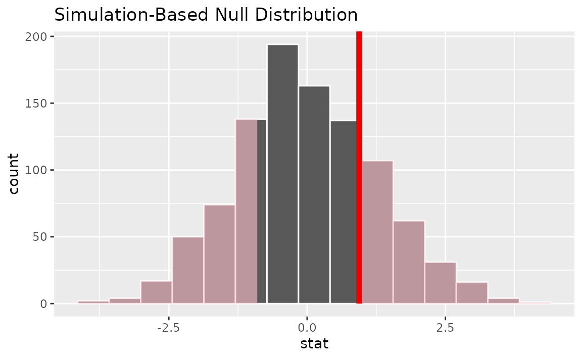
Calculating the p-value from the null distribution and observed statistic,
null_dist |>
  get_p_value(obs_stat = d_hat, direction = "two-sided")
## # A tibble: 1 × 1
## p_value
## <dbl>
## 1 0.46One numerical variable, one categorical (2 levels) (t)
Finding the standardized observed statistic,
t_hat <- gss |>
  specify(age ~ college) |>
  hypothesize(null = "independence") |>
  calculate(stat = "t", order = c("degree", "no degree"))
Alternatively, using the observe() wrapper to calculate
the observed statistic,
Then, generating the null distribution,
null_dist <- gss |>
  specify(age ~ college) |>
  hypothesize(null = "independence") |>
  generate(reps = 1000, type = "permute") |>
  calculate(stat = "t", order = c("degree", "no degree"))
Alternatively, finding the null distribution using theoretical
methods using the assume() verb,
Visualizing the observed statistic alongside the null distribution,
visualize(null_dist) +
  shade_p_value(obs_stat = t_hat, direction = "two-sided")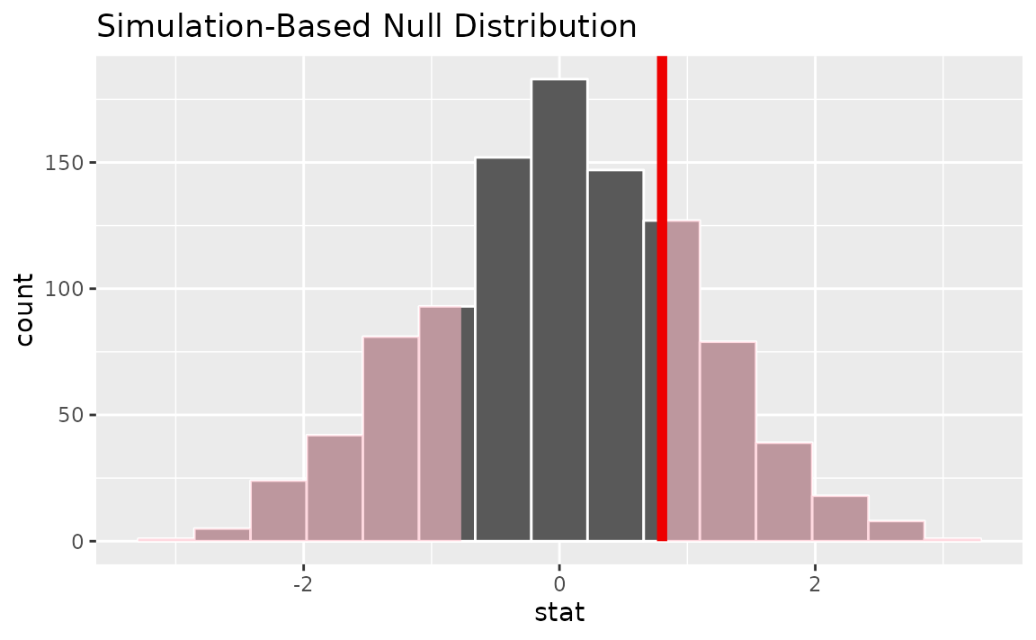
Alternatively, visualizing the observed statistic using the theory-based null distribution,
visualize(null_dist_theory) +
  shade_p_value(obs_stat = t_hat, direction = "two-sided")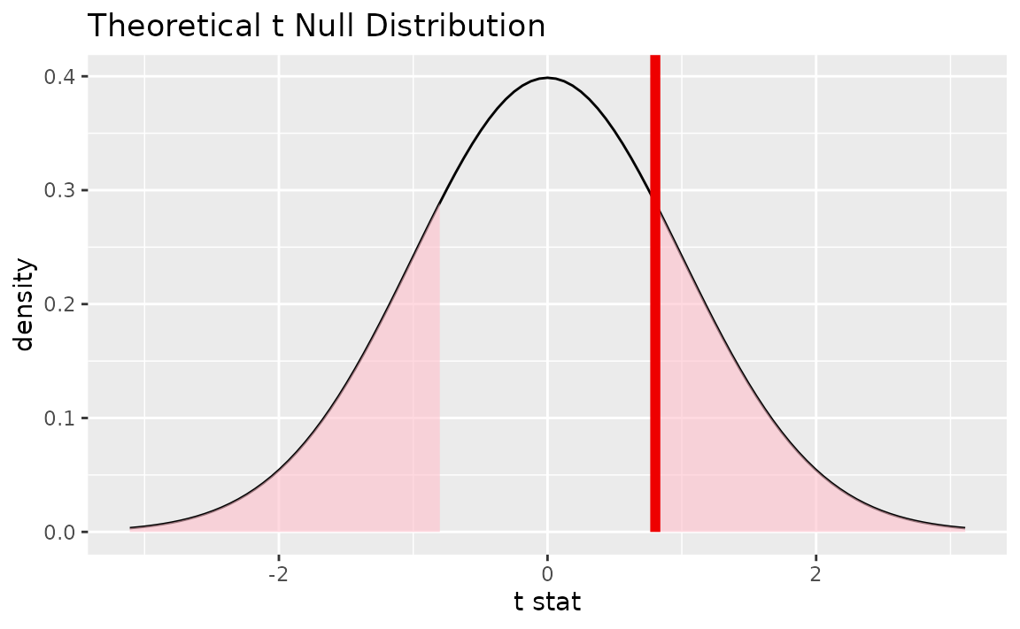
Alternatively, visualizing the observed statistic using both of the null distributions,
visualize(null_dist, method = "both") +
  shade_p_value(obs_stat = t_hat, direction = "two-sided")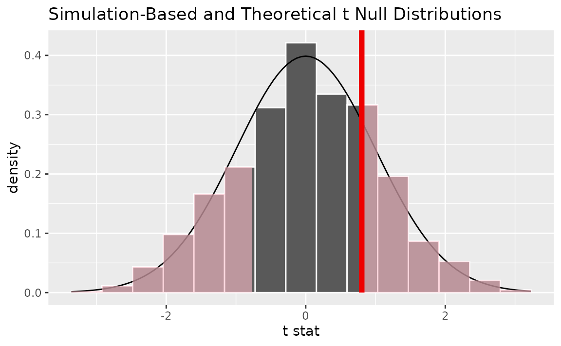
Note that the above code makes use of the randomization-based null distribution.
Calculating the p-value from the null distribution and observed statistic,
null_dist |>
  get_p_value(obs_stat = t_hat, direction = "two-sided")
## # A tibble: 1 × 1
## p_value
## <dbl>
## 1 0.442Note the similarities in this plot and the previous one.
One numerical variable, one categorical (2 levels) (diff in medians)
Calculating the observed statistic,
d_hat <- gss |>
  specify(age ~ college) |>
  calculate(stat = "diff in medians", order = c("degree", "no degree"))
Alternatively, using the observe() wrapper to calculate
the observed statistic,
Then, generating the null distribution,
null_dist <- gss |>
  specify(age ~ college) |> # alt: response = age, explanatory = season
  hypothesize(null = "independence") |>
  generate(reps = 1000, type = "permute") |>
  calculate(stat = "diff in medians", order = c("degree", "no degree"))
Visualizing the observed statistic alongside the null distribution,
visualize(null_dist) +
  shade_p_value(obs_stat = d_hat, direction = "two-sided")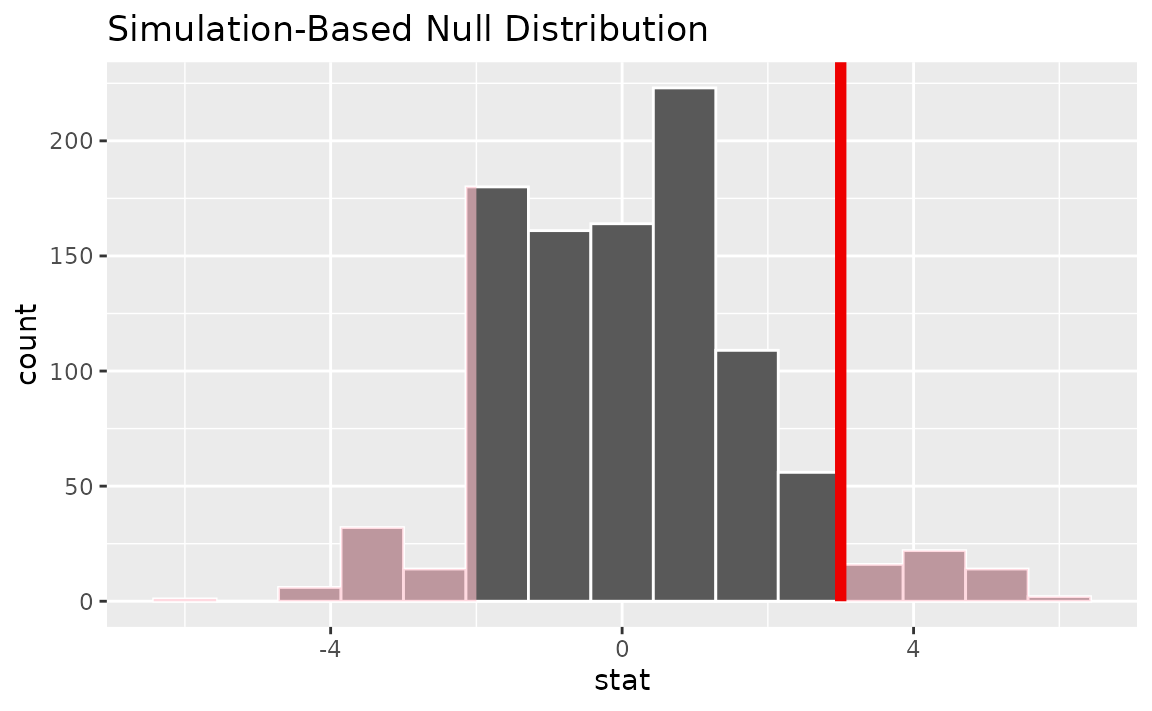
Calculating the p-value from the null distribution and observed statistic,
null_dist |>
  get_p_value(obs_stat = d_hat, direction = "two-sided")
## # A tibble: 1 × 1
## p_value
## <dbl>
## 1 0.172One numerical, one categorical (>2 levels) - ANOVA
Calculating the observed statistic,
Alternatively, using the observe() wrapper to calculate
the observed statistic,
F_hat <- gss |>
  observe(age ~ partyid, stat = "F")
Then, generating the null distribution,
null_dist <- gss |>
   specify(age ~ partyid) |>
   hypothesize(null = "independence") |>
   generate(reps = 1000, type = "permute") |>
   calculate(stat = "F")
Alternatively, finding the null distribution using theoretical
methods using the assume() verb,
null_dist_theory <- gss |>
   specify(age ~ partyid) |>
   hypothesize(null = "independence") |>
   assume(distribution = "F")
Visualizing the observed statistic alongside the null distribution,
visualize(null_dist) +
  shade_p_value(obs_stat = F_hat, direction = "greater")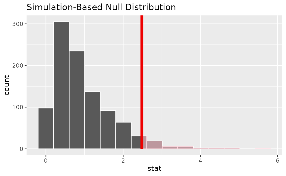
Alternatively, visualizing the observed statistic using the theory-based null distribution,
visualize(null_dist_theory) +
  shade_p_value(obs_stat = F_hat, direction = "greater")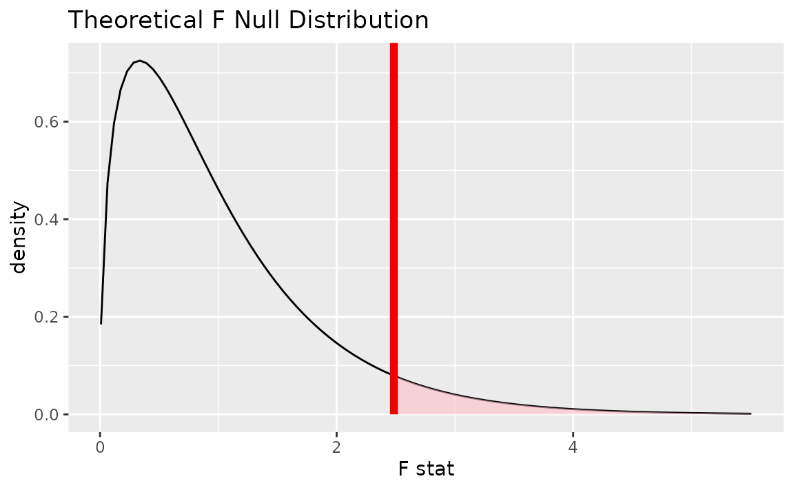
Alternatively, visualizing the observed statistic using both of the null distributions,
visualize(null_dist, method = "both") +
  shade_p_value(obs_stat = F_hat, direction = "greater")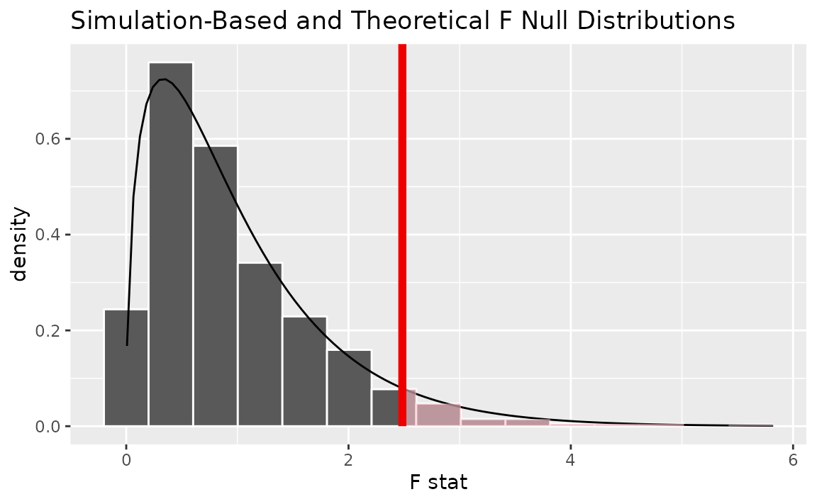
Note that the above code makes use of the randomization-based null distribution.
Calculating the p-value from the null distribution and observed statistic,
null_dist |>
  get_p_value(obs_stat = F_hat, direction = "greater")
## # A tibble: 1 × 1
## p_value
## <dbl>
## 1 0.045Two numerical vars - SLR
Calculating the observed statistic,
Alternatively, using the observe() wrapper to calculate
the observed statistic,
slope_hat <- gss |>
  observe(hours ~ age, stat = "slope")
Then, generating the null distribution,
null_dist <- gss |>
   specify(hours ~ age) |>
   hypothesize(null = "independence") |>
   generate(reps = 1000, type = "permute") |>
   calculate(stat = "slope")
Visualizing the observed statistic alongside the null distribution,
visualize(null_dist) +
  shade_p_value(obs_stat = slope_hat, direction = "two-sided")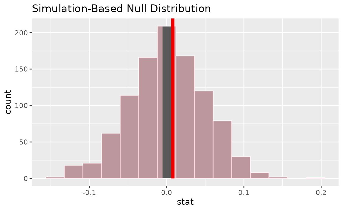
Calculating the p-value from the null distribution and observed statistic,
null_dist |>
  get_p_value(obs_stat = slope_hat, direction = "two-sided")
## # A tibble: 1 × 1
## p_value
## <dbl>
## 1 0.902Two numerical vars - correlation
Calculating the observed statistic,
Alternatively, using the observe() wrapper to calculate
the observed statistic,
correlation_hat <- gss |>
  observe(hours ~ age, stat = "correlation")
Then, generating the null distribution,
null_dist <- gss |>
   specify(hours ~ age) |>
   hypothesize(null = "independence") |>
   generate(reps = 1000, type = "permute") |>
   calculate(stat = "correlation")
Visualizing the observed statistic alongside the null distribution,
visualize(null_dist) +
  shade_p_value(obs_stat = correlation_hat, direction = "two-sided")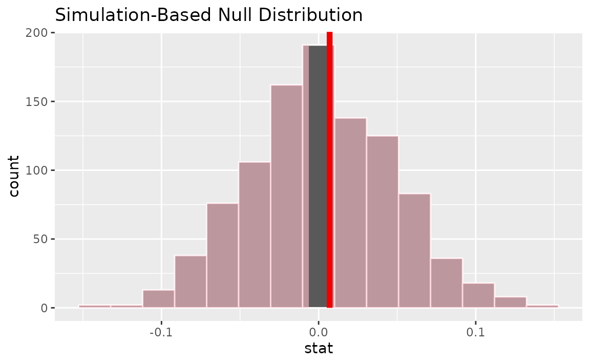
Calculating the p-value from the null distribution and observed statistic,
null_dist |>
  get_p_value(obs_stat = correlation_hat, direction = "two-sided")
## # A tibble: 1 × 1
## p_value
## <dbl>
## 1 0.878Two numerical vars - SLR (t)
Not currently implemented since could refer to standardized slope or standardized correlation.
Multiple explanatory variables
Calculating the observed fit,
Generating a distribution of fits with the response variable permuted,
null_dist <- gss |>
  specify(hours ~ age + college) |>
  hypothesize(null = "independence") |>
  generate(reps = 1000, type = "permute") |>
  fit()
Generating a distribution of fits where each explanatory variable is permuted independently,
null_dist2 <- gss |>
  specify(hours ~ age + college) |>
  hypothesize(null = "independence") |>
  generate(reps = 1000, type = "permute", variables = c(age, college)) |>
  fit()
Visualizing the observed fit alongside the null fits,
visualize(null_dist) +
  shade_p_value(obs_stat = obs_fit, direction = "two-sided")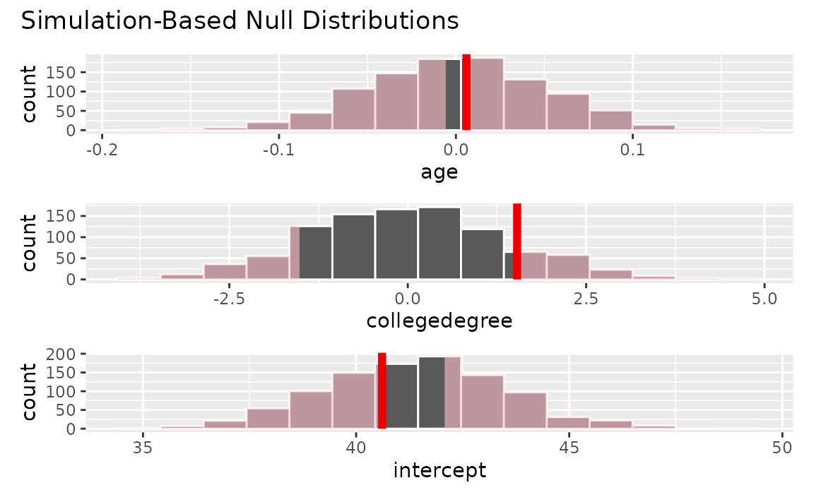
Calculating p-values from the null distribution and observed fit,
null_dist |>
  get_p_value(obs_stat = obs_fit, direction = "two-sided")
## # A tibble: 3 × 2
## term p_value
## <chr> <dbl>
## 1 age 0.914
## 2 collegedegree 0.266
## 3 intercept 0.734Note that this fit()-based workflow can be applied to
use cases with differing numbers of explanatory variables and
explanatory variable types.
Confidence intervals
One numerical (one mean)
Finding the observed statistic,
Alternatively, using the observe() wrapper to calculate
the observed statistic,
x_bar <- gss |>
  observe(response = hours, stat = "mean")
Then, generating a bootstrap distribution,
boot_dist <- gss |>
   specify(response = hours) |>
   generate(reps = 1000, type = "bootstrap") |>
   calculate(stat = "mean")
Use the bootstrap distribution to find a confidence interval,
percentile_ci <- get_ci(boot_dist)Visualizing the observed statistic alongside the distribution,
visualize(boot_dist) +
  shade_confidence_interval(endpoints = percentile_ci)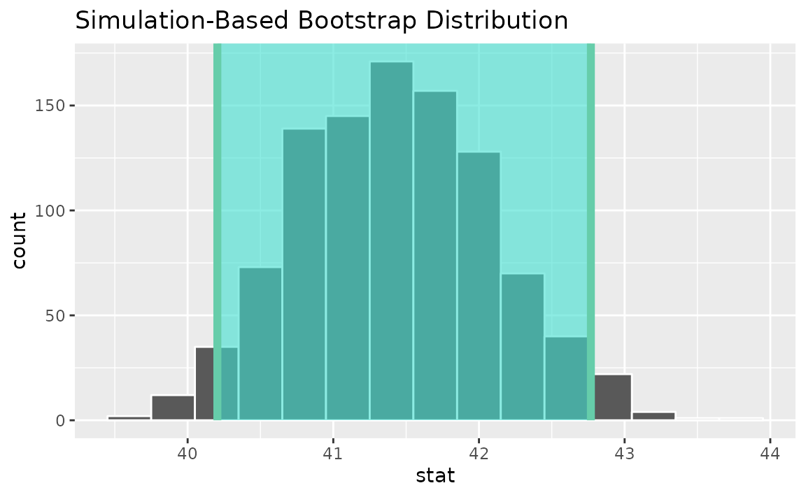
Alternatively, use the bootstrap distribution to find a confidence interval using the standard error,
standard_error_ci <- get_ci(boot_dist, type = "se", point_estimate = x_bar)

visualize(boot_dist) +
  shade_confidence_interval(endpoints = standard_error_ci)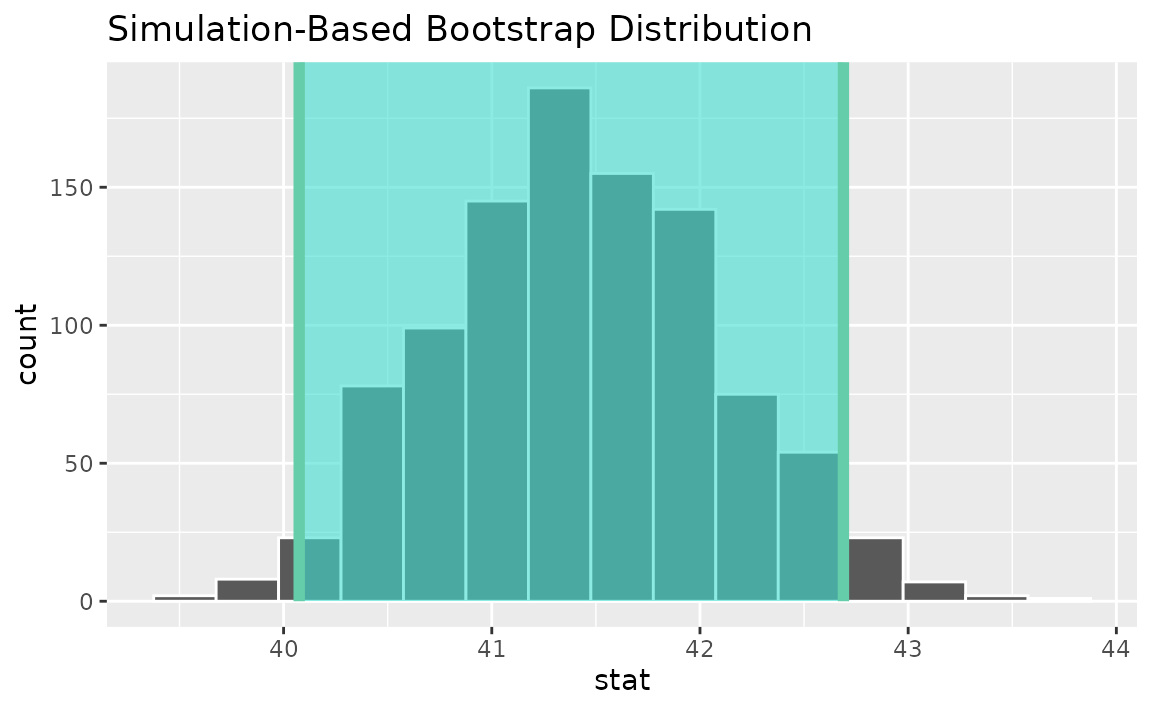
Instead of a simulation-based bootstrap distribution, we can also define a theory-based sampling distribution,
Visualization and calculation of confidence intervals interfaces in the same way as with the simulation-based distribution,
theor_ci <- get_ci(sampling_dist, point_estimate = x_bar)

theor_ci
## # A tibble: 1 × 2
## lower_ci upper_ci
## <dbl> <dbl>
## 1 40.1 42.7
visualize(sampling_dist) +
  shade_confidence_interval(endpoints = theor_ci)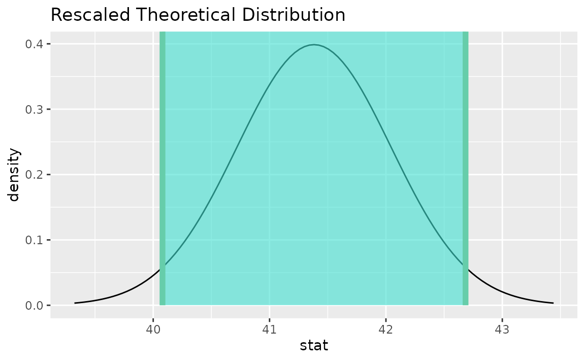
Note that the t distribution is recentered and rescaled
to lie on the scale of the observed data. infer does not support
confidence intervals on means via the z distribution.
One numerical (one mean - standardized)
Finding the observed statistic,
t_hat <- gss |>
  specify(response = hours) |>
  hypothesize(null = "point", mu = 40) |>
  calculate(stat = "t")
Alternatively, using the observe() wrapper to calculate
the observed statistic,
t_hat <- gss |>
  observe(response = hours,
          null = "point", mu = 40,
          stat = "t")
Then, generating the bootstrap distribution,
boot_dist <- gss |>
   specify(response = hours) |>
   generate(reps = 1000, type = "bootstrap") |>
   calculate(stat = "t")
Use the bootstrap distribution to find a confidence interval,
percentile_ci <- get_ci(boot_dist)Visualizing the observed statistic alongside the distribution,
visualize(boot_dist) +
  shade_confidence_interval(endpoints = percentile_ci)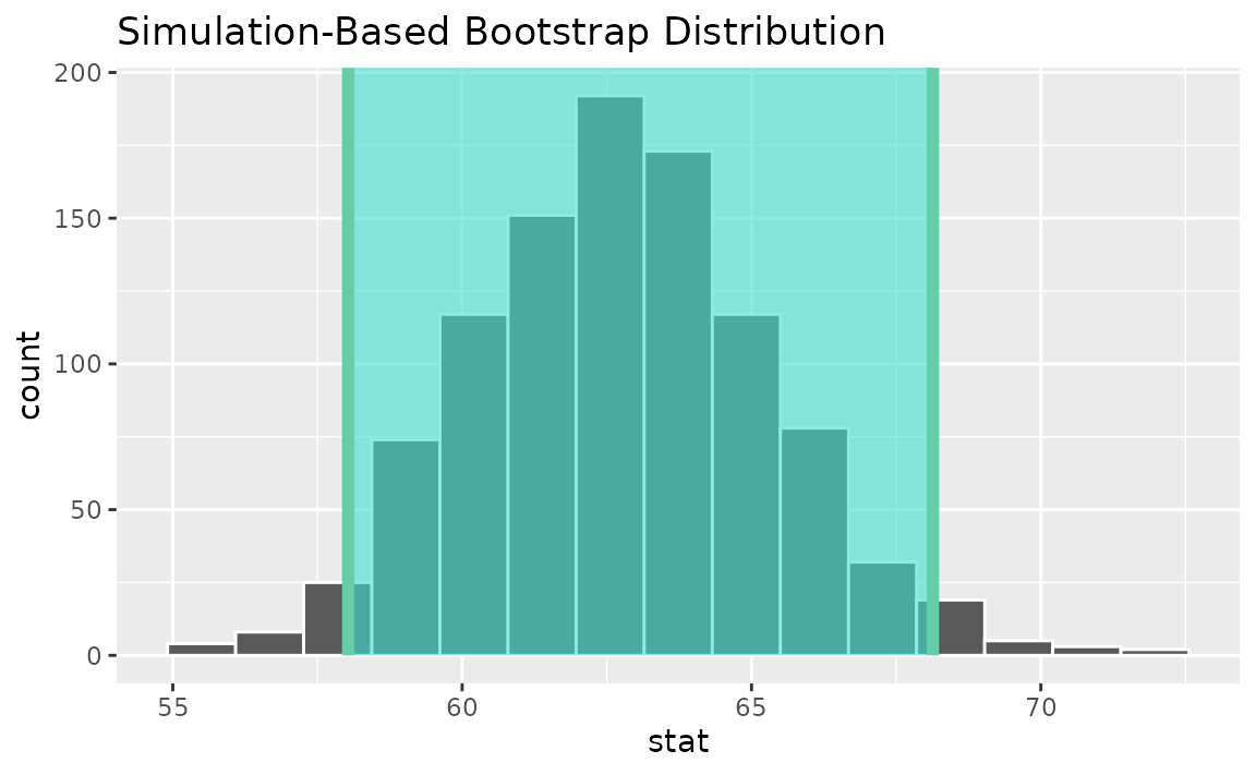
Alternatively, use the bootstrap distribution to find a confidence interval using the standard error,
standard_error_ci <- boot_dist |>
  get_ci(type = "se", point_estimate = t_hat)

visualize(boot_dist) +
  shade_confidence_interval(endpoints = standard_error_ci)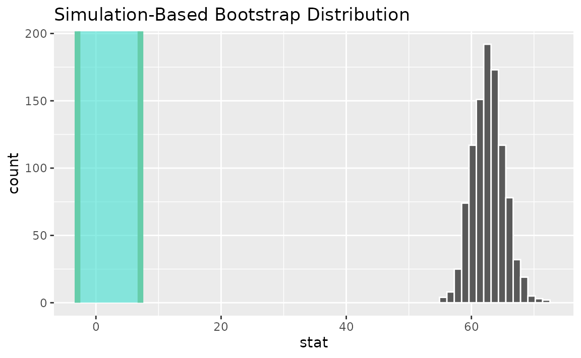
See the above subsection (one mean) for a theory-based approach. Note
that infer does not support confidence intervals on means via the
z distribution.
One categorical (one proportion)
Finding the observed statistic,
Alternatively, using the observe() wrapper to calculate
the observed statistic,
p_hat <- gss |>
   observe(response = sex, success = "female", stat = "prop")
Then, generating a bootstrap distribution,
boot_dist <- gss |>
 specify(response = sex, success = "female") |>
 generate(reps = 1000, type = "bootstrap") |>
 calculate(stat = "prop")
Use the bootstrap distribution to find a confidence interval,
percentile_ci <- get_ci(boot_dist)Visualizing the observed statistic alongside the distribution,
visualize(boot_dist) +
  shade_confidence_interval(endpoints = percentile_ci)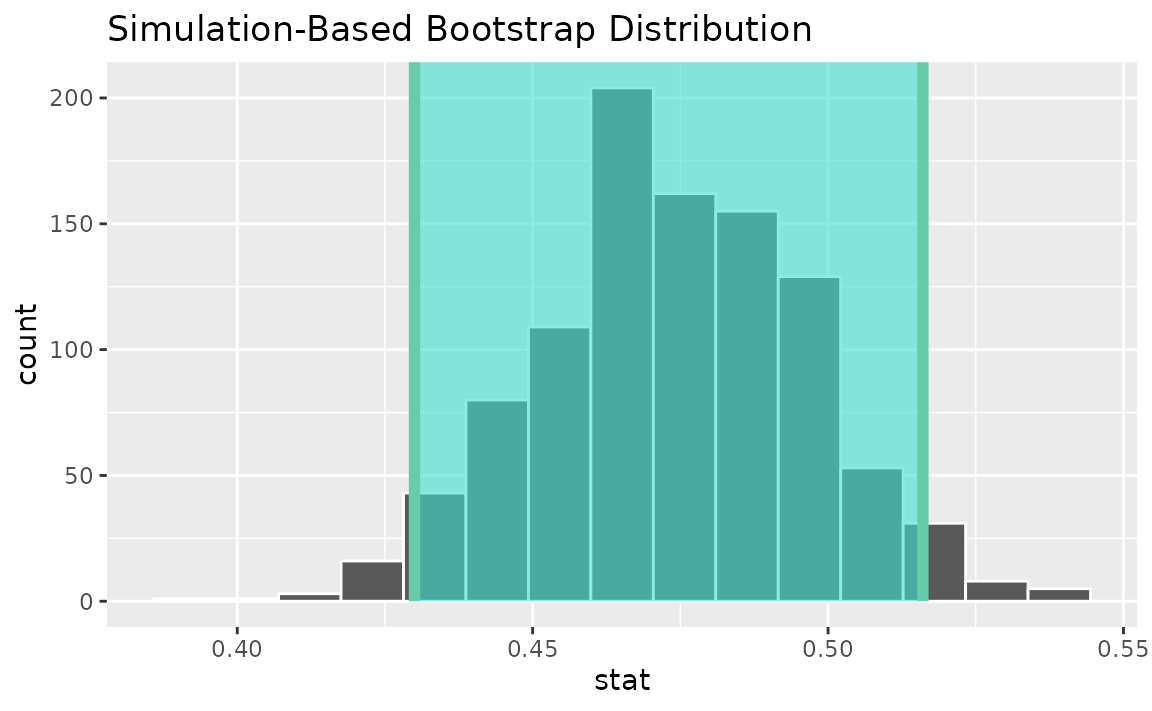
Alternatively, use the bootstrap distribution to find a confidence interval using the standard error,
standard_error_ci <- boot_dist |>
  get_ci(type = "se", point_estimate = p_hat)

visualize(boot_dist) +
  shade_confidence_interval(endpoints = standard_error_ci)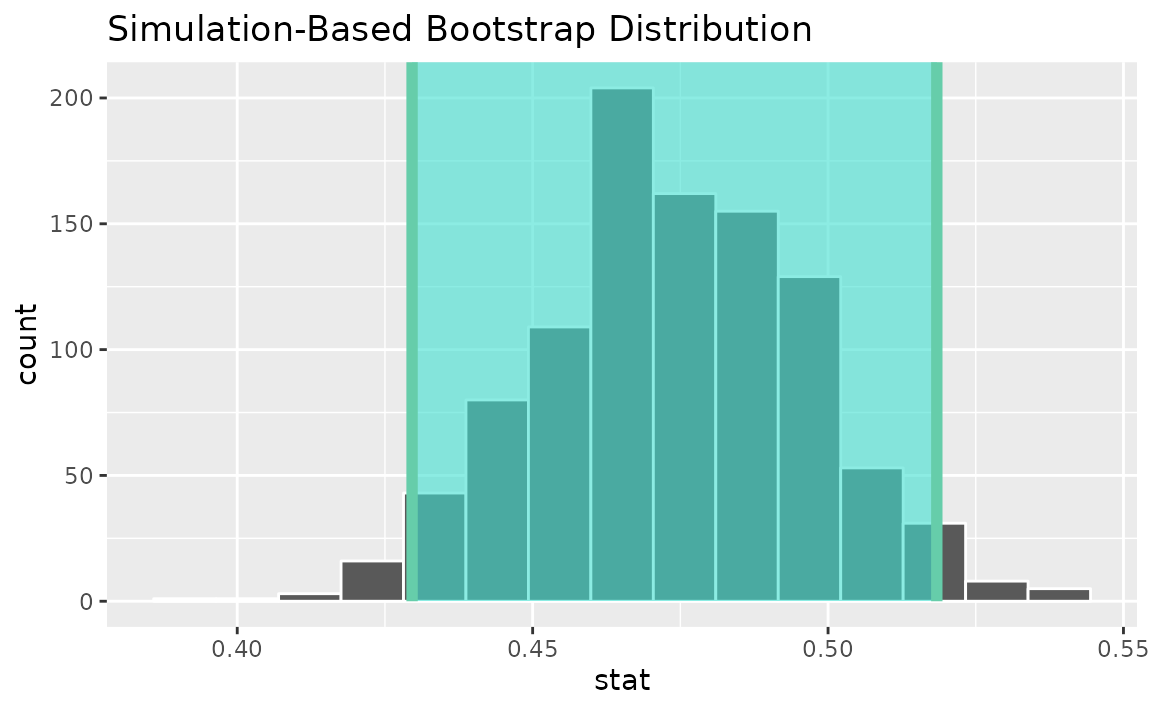
Instead of a simulation-based bootstrap distribution, we can also define a theory-based sampling distribution,
Visualization and calculation of confidence intervals interfaces in the same way as with the simulation-based distribution,
theor_ci <- get_ci(sampling_dist, point_estimate = p_hat)

theor_ci
## # A tibble: 1 × 2
## lower_ci upper_ci
## <dbl> <dbl>
## 1 0.430 0.518
visualize(sampling_dist) +
  shade_confidence_interval(endpoints = theor_ci)
Note that the z distribution is recentered and rescaled
to lie on the scale of the observed data. infer does not
support confidence intervals on means via the z
distribution.
One categorical variable (standardized proportion )
See the above subsection (one proportion) for a theory-based approach.
One numerical variable, one categorical (2 levels) (diff in means)
Finding the observed statistic,
d_hat <- gss |>
  specify(hours ~ college) |>
  calculate(stat = "diff in means", order = c("degree", "no degree"))
Alternatively, using the observe() wrapper to calculate
the observed statistic,
Then, generating a bootstrap distribution,
boot_dist <- gss |>
   specify(hours ~ college) |>
   generate(reps = 1000, type = "bootstrap") |>
   calculate(stat = "diff in means", order = c("degree", "no degree"))
Use the bootstrap distribution to find a confidence interval,
percentile_ci <- get_ci(boot_dist)Visualizing the observed statistic alongside the distribution,
visualize(boot_dist) +
  shade_confidence_interval(endpoints = percentile_ci)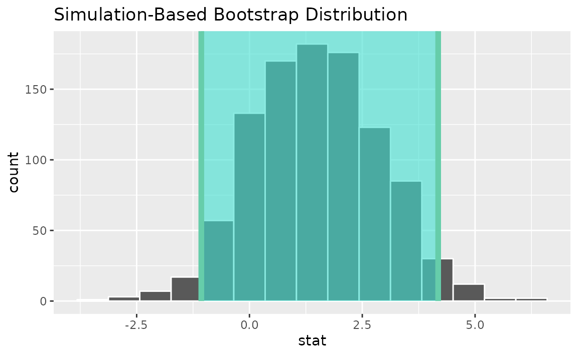
Alternatively, use the bootstrap distribution to find a confidence interval using the standard error,
standard_error_ci <- boot_dist |>
  get_ci(type = "se", point_estimate = d_hat)

visualize(boot_dist) +
  shade_confidence_interval(endpoints = standard_error_ci)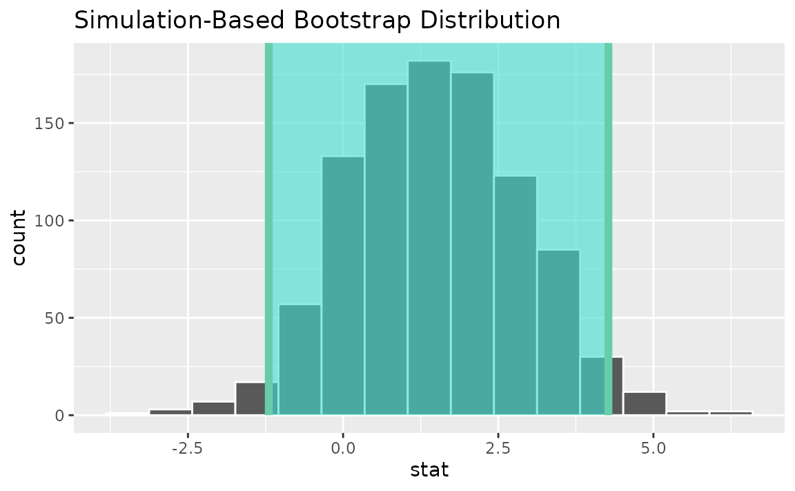
Instead of a simulation-based bootstrap distribution, we can also define a theory-based sampling distribution,
Visualization and calculation of confidence intervals interfaces in the same way as with the simulation-based distribution,
theor_ci <- get_ci(sampling_dist, point_estimate = d_hat)

theor_ci
## # A tibble: 1 × 2
## lower_ci upper_ci
## <dbl> <dbl>
## 1 -1.16 4.24
visualize(sampling_dist) +
  shade_confidence_interval(endpoints = theor_ci)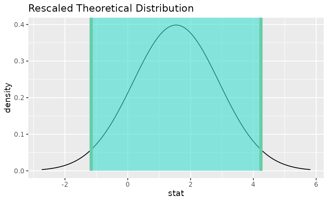
Note that the t distribution is recentered and rescaled
to lie on the scale of the observed data.
infer also provides functionality to calculate ratios of
means. The workflow looks similar to that for
diff in means.
Finding the observed statistic,
d_hat <- gss |>
  specify(hours ~ college) |>
  calculate(stat = "ratio of means", order = c("degree", "no degree"))
Alternatively, using the observe() wrapper to calculate
the observed statistic,
Then, generating a bootstrap distribution,
boot_dist <- gss |>
   specify(hours ~ college) |>
   generate(reps = 1000, type = "bootstrap") |>
   calculate(stat = "ratio of means", order = c("degree", "no degree"))
Use the bootstrap distribution to find a confidence interval,
percentile_ci <- get_ci(boot_dist)Visualizing the observed statistic alongside the distribution,
visualize(boot_dist) +
  shade_confidence_interval(endpoints = percentile_ci)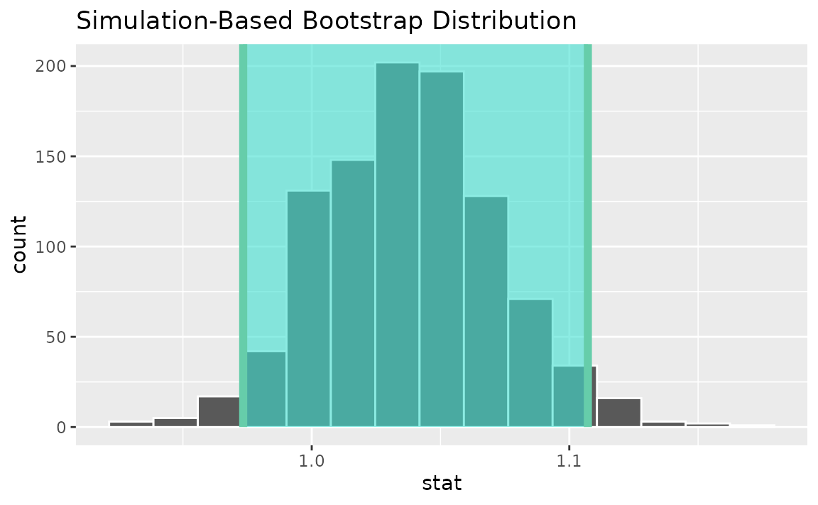
Alternatively, use the bootstrap distribution to find a confidence interval using the standard error,
standard_error_ci <- boot_dist |>
  get_ci(type = "se", point_estimate = d_hat)

visualize(boot_dist) +
  shade_confidence_interval(endpoints = standard_error_ci)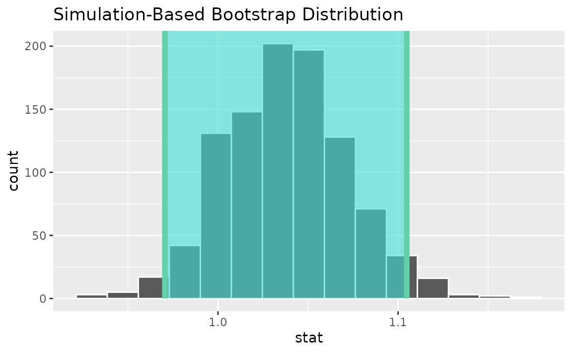
One numerical variable, one categorical (2 levels) (t)
Finding the standardized point estimate,
Alternatively, using the observe() wrapper to calculate
the observed statistic,
Then, generating a bootstrap distribution,
boot_dist <- gss |>
   specify(hours ~ college) |>
   generate(reps = 1000, type = "bootstrap") |>
   calculate(stat = "t", order = c("degree", "no degree"))
Use the bootstrap distribution to find a confidence interval,
percentile_ci <- get_ci(boot_dist)Visualizing the observed statistic alongside the distribution,
visualize(boot_dist) +
  shade_confidence_interval(endpoints = percentile_ci)
Alternatively, use the bootstrap distribution to find a confidence interval using the standard error,
standard_error_ci <- boot_dist |>
  get_ci(type = "se", point_estimate = t_hat)

visualize(boot_dist) +
  shade_confidence_interval(endpoints = standard_error_ci)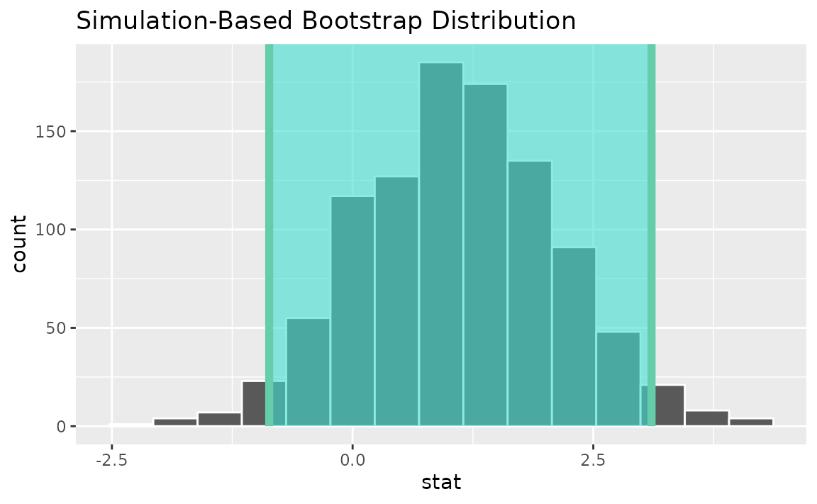
See the above subsection (diff in means) for a theory-based approach.
infer does not support confidence intervals on means via
the z distribution.
Two categorical variables (diff in proportions)
Finding the observed statistic,
d_hat <- gss |>
  specify(college ~ sex, success = "degree") |>
  calculate(stat = "diff in props", order = c("female", "male"))
Alternatively, using the observe() wrapper to calculate
the observed statistic,
d_hat <- gss |>
  observe(college ~ sex, success = "degree",
          stat = "diff in props", order = c("female", "male"))
Then, generating a bootstrap distribution,
boot_dist <- gss |>
  specify(college ~ sex, success = "degree") |>
  generate(reps = 1000, type = "bootstrap") |>
  calculate(stat = "diff in props", order = c("female", "male"))
Use the bootstrap distribution to find a confidence interval,
percentile_ci <- get_ci(boot_dist)Visualizing the observed statistic alongside the distribution,
visualize(boot_dist) +
  shade_confidence_interval(endpoints = percentile_ci)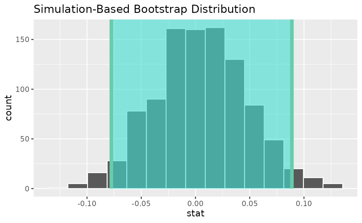
Alternatively, use the bootstrap distribution to find a confidence interval using the standard error,
standard_error_ci <- boot_dist |>
  get_ci(type = "se", point_estimate = d_hat)

visualize(boot_dist) +
  shade_confidence_interval(endpoints = standard_error_ci)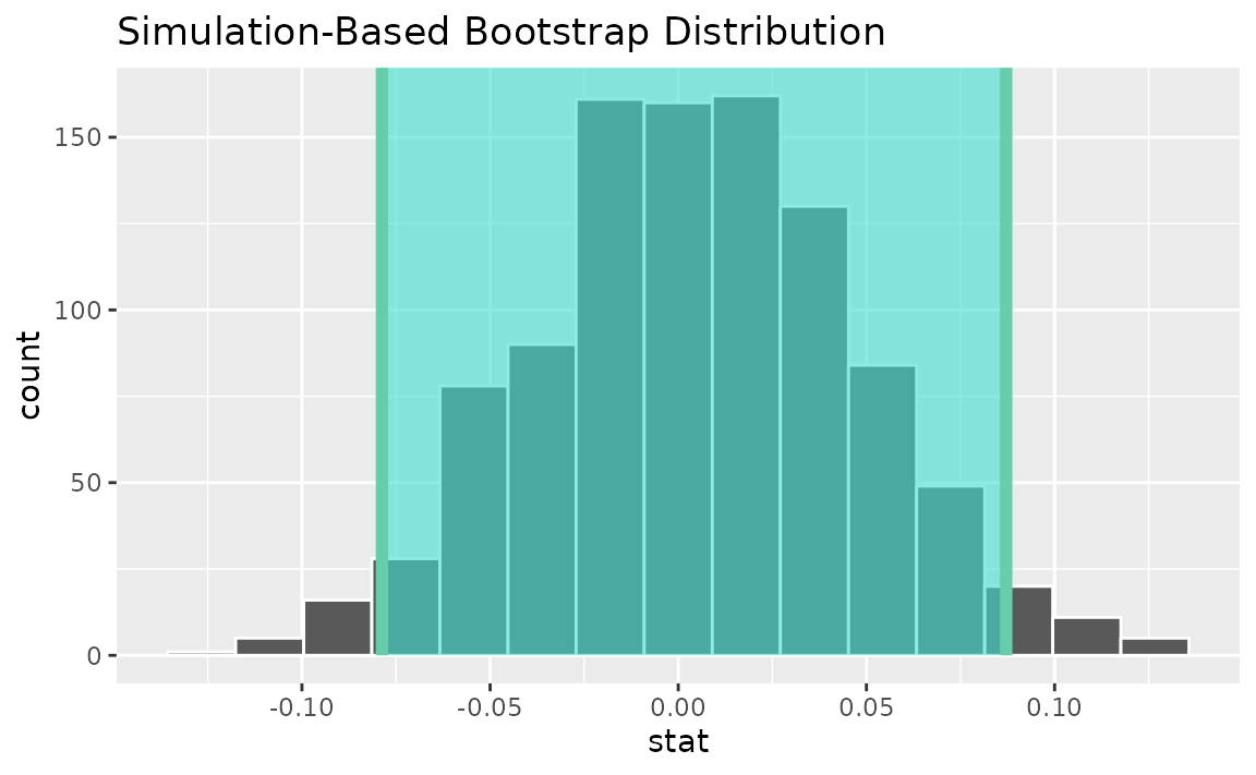
Instead of a simulation-based bootstrap distribution, we can also define a theory-based sampling distribution,
Visualization and calculation of confidence intervals interfaces in the same way as with the simulation-based distribution,
theor_ci <- get_ci(sampling_dist, point_estimate = d_hat)

theor_ci
## # A tibble: 1 × 2
## lower_ci upper_ci
## <dbl> <dbl>
## 1 -0.0794 0.0878
visualize(sampling_dist) +
  shade_confidence_interval(endpoints = theor_ci)
Note that the z distribution is recentered and rescaled
to lie on the scale of the observed data.
Two categorical variables (z)
Finding the standardized point estimate,
z_hat <- gss |>
  specify(college ~ sex, success = "degree") |>
  calculate(stat = "z", order = c("female", "male"))
Alternatively, using the observe() wrapper to calculate
the observed statistic,
Then, generating a bootstrap distribution,
boot_dist <- gss |>
  specify(college ~ sex, success = "degree") |>
  generate(reps = 1000, type = "bootstrap") |>
  calculate(stat = "z", order = c("female", "male"))
Use the bootstrap distribution to find a confidence interval,
percentile_ci <- get_ci(boot_dist)Visualizing the observed statistic alongside the distribution,
visualize(boot_dist) +
shade_confidence_interval(endpoints = percentile_ci)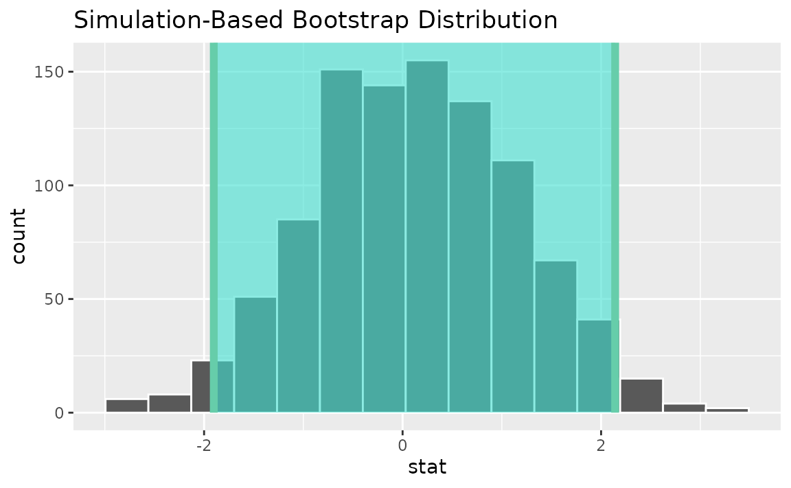
Alternatively, use the bootstrap distribution to find a confidence interval using the standard error,
standard_error_ci <- boot_dist |>
get_ci(type = "se", point_estimate = z_hat)
visualize(boot_dist) +
shade_confidence_interval(endpoints = standard_error_ci)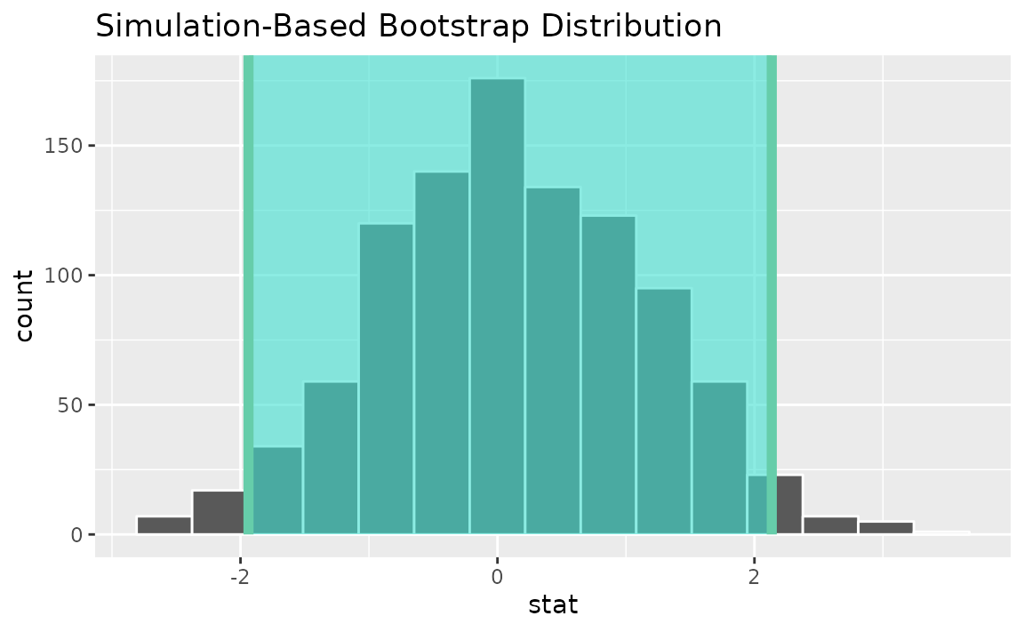
See the above subsection (diff in props) for a theory-based approach.
Two numerical vars - SLR
Finding the observed statistic,
Alternatively, using the observe() wrapper to calculate
the observed statistic,
slope_hat <- gss |>
observe(hours ~ age, stat = "slope")Then, generating a bootstrap distribution,
boot_dist <- gss |>
specify(hours ~ age) |>
generate(reps = 1000, type = "bootstrap") |>
calculate(stat = "slope")Use the bootstrap distribution to find a confidence interval,
percentile_ci <- get_ci(boot_dist)Visualizing the observed statistic alongside the distribution,
visualize(boot_dist) +
shade_confidence_interval(endpoints = percentile_ci)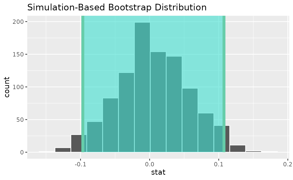
Alternatively, use the bootstrap distribution to find a confidence interval using the standard error,
standard_error_ci <- boot_dist |>
get_ci(type = "se", point_estimate = slope_hat)
visualize(boot_dist) +
shade_confidence_interval(endpoints = standard_error_ci)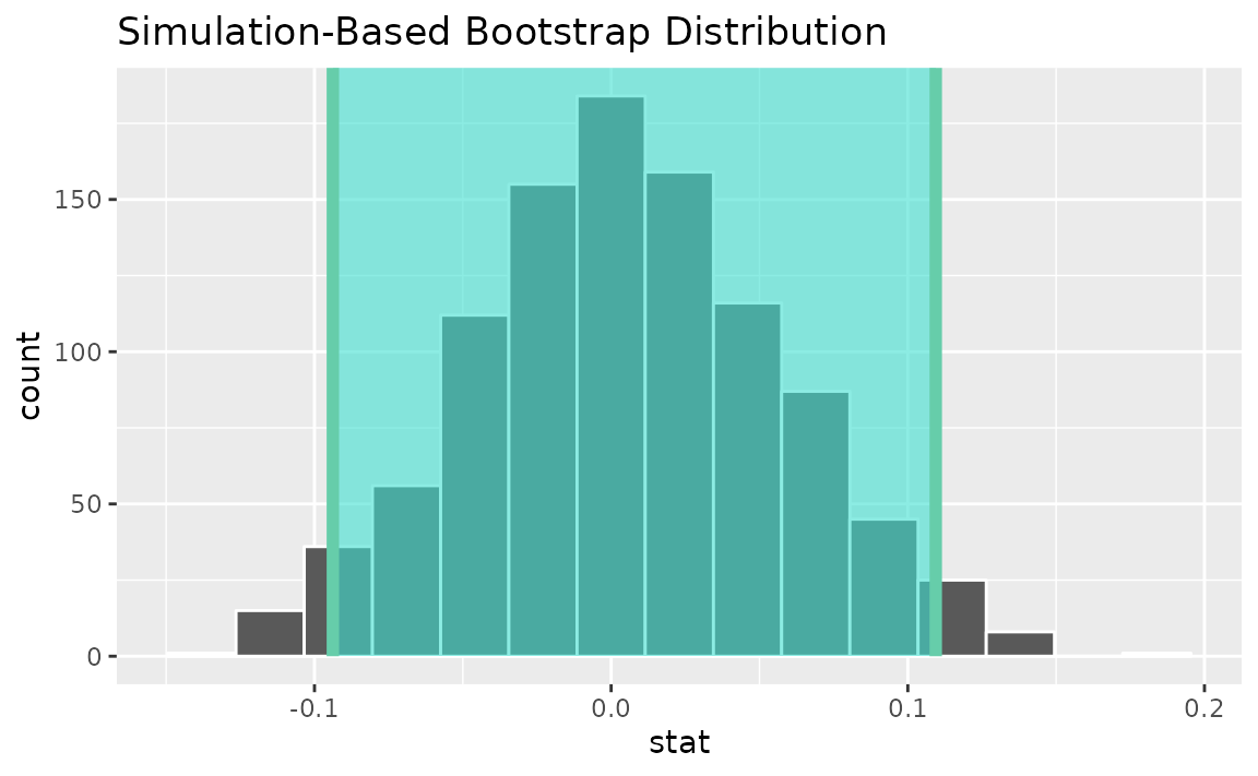
Two numerical vars - correlation
Finding the observed statistic,
Alternatively, using the observe() wrapper to calculate
the observed statistic,
correlation_hat <- gss |>
observe(hours ~ age, stat = "correlation")Then, generating a bootstrap distribution,
boot_dist <- gss |>
specify(hours ~ age) |>
generate(reps = 1000, type = "bootstrap") |>
calculate(stat = "correlation")Use the bootstrap distribution to find a confidence interval,
percentile_ci <- get_ci(boot_dist)Visualizing the observed statistic alongside the distribution,
visualize(boot_dist) +
shade_confidence_interval(endpoints = percentile_ci)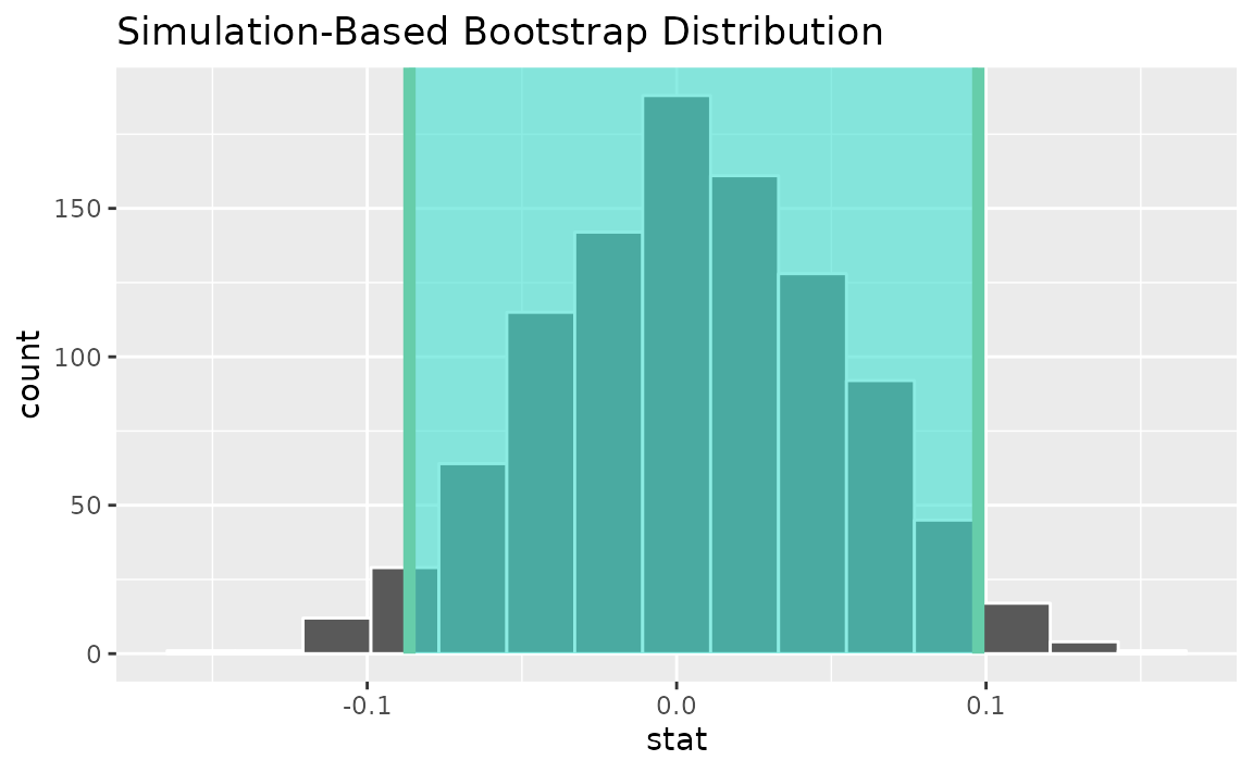
Alternatively, use the bootstrap distribution to find a confidence interval using the standard error,
standard_error_ci <- boot_dist |>
get_ci(type = "se", point_estimate = correlation_hat)
visualize(boot_dist) +
shade_confidence_interval(endpoints = standard_error_ci)
Two numerical vars - t
Not currently implemented since could refer to standardized slope or standardized correlation.
Multiple explanatory variables
Calculating the observed fit,
Then, generating a bootstrap distribution,
boot_dist <- gss |>
specify(hours ~ age + college) |>
generate(reps = 1000, type = "bootstrap") |>
fit()Use the bootstrap distribution to find a confidence interval,
conf_ints <-
get_confidence_interval(
boot_dist,
level = .95,
point_estimate = obs_fit
)Visualizing the observed statistic alongside the distribution,
visualize(boot_dist) +
shade_confidence_interval(endpoints = conf_ints)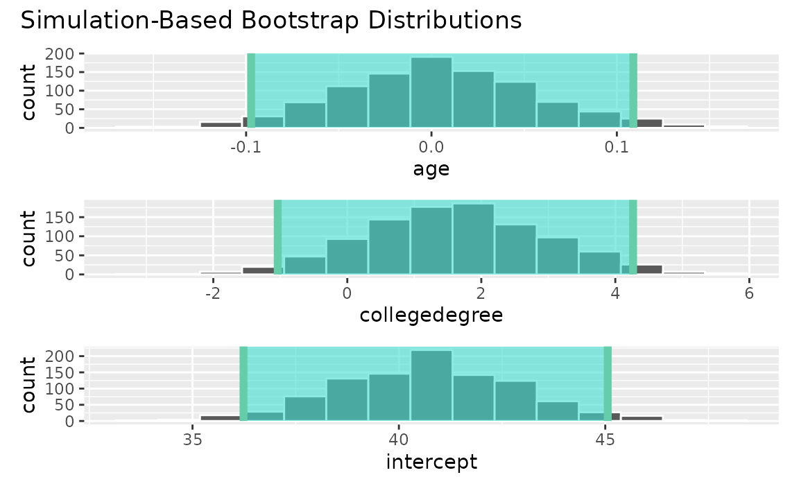
Note that this fit()-based workflow can be applied to
use cases with differing numbers of explanatory variables and
explanatory variable types.