Perform repeated sampling — rep_sample

These functions extend the functionality of dplyr::sample_n() and dplyr::slice_sample() by allowing for repeated sampling of data. This operation is especially helpful while creating sampling distributions—see the examples below!

rep_sample_n(tbl, size, replace = FALSE, reps = 1, prob = NULL)

rep_slice_sample(
  .data,
  n = NULL,
  prop = NULL,
  replace = FALSE,
  weight_by = NULL,
  reps = 1
)

Arguments

tbl, .data	Data frame of population from which to sample.
size, n, prop	`size` and `n` refer to the sample size of each sample. The `size` argument to `rep_sample_n()` is required, while in `rep_slice_sample()` sample size defaults to 1 if not specified. `prop`, an argument to `rep_slice_sample()`, refers to the proportion of rows to sample in each sample, and is rounded down in the case that `prop * nrow(.data)` is not an integer. When using `rep_slice_sample()`, please only supply one of `n` or `prop`.
replace	Should samples be taken with replacement?
reps	Number of samples to take.
prob, weight_by	A vector of sampling weights for each of the rows in `.data`—must have length equal to `nrow(.data)`.

Value

A tibble of size reps * n rows corresponding to reps samples of size n from .data, grouped by replicate.

Details

rep_sample_n() and rep_slice_sample() are designed to behave similar to their dplyr counterparts. As such, they have at least the following differences:

In case replace = FALSE having size bigger than number of data rows in rep_sample_n() will give an error. In rep_slice_sample() having such n or prop > 1 will give warning and output sample size will be set to number of rows in data.

Note that the dplyr::sample_n() function has been superseded by dplyr::slice_sample().

Examples

library(dplyr)
#> 
#> Attaching package: ‘dplyr’
#> The following objects are masked from ‘package:stats’:
#> 
#>     filter, lag
#> The following objects are masked from ‘package:base’:
#> 
#>     intersect, setdiff, setequal, union
library(ggplot2)
library(tibble)

# take 1000 samples of size n = 50, without replacement
slices <- gss %>%
  rep_slice_sample(n = 50, reps = 1000)

slices
#> # A tibble: 50,000 × 12
#> # Groups:   replicate [1,000]
#>    replicate  year   age sex   college partyid hompop hours income class finrela
#>        <int> <dbl> <dbl> <fct> <fct>   <fct>    <dbl> <dbl> <ord>  <fct> <fct>  
#>  1         1  1998    27 fema… no deg… rep          3    40 $1500… work… average
#>  2         1  2012    26 fema… no deg… ind         10    20 $2500… work… below …
#>  3         1  1996    54 male  no deg… ind          4    30 $1500… work… below …
#>  4         1  1993    39 fema… no deg… ind          6    37 $2000… work… average
#>  5         1  2010    49 male  degree  ind          1    40 $2500… midd… average
#>  6         1  1991    27 fema… degree  rep          1    50 $2500… midd… average
#>  7         1  1985    38 fema… no deg… dem          4    38 $8000… lowe… far be…
#>  8         1  2000    37 male  no deg… dem          3    50 $2500… work… average
#>  9         1  2000    22 male  no deg… ind          2    15 $4000… midd… average
#> 10         1  1998    45 male  degree  rep          1    50 $2500… midd… average
#> # … with 49,990 more rows, and 1 more variable: weight <dbl>

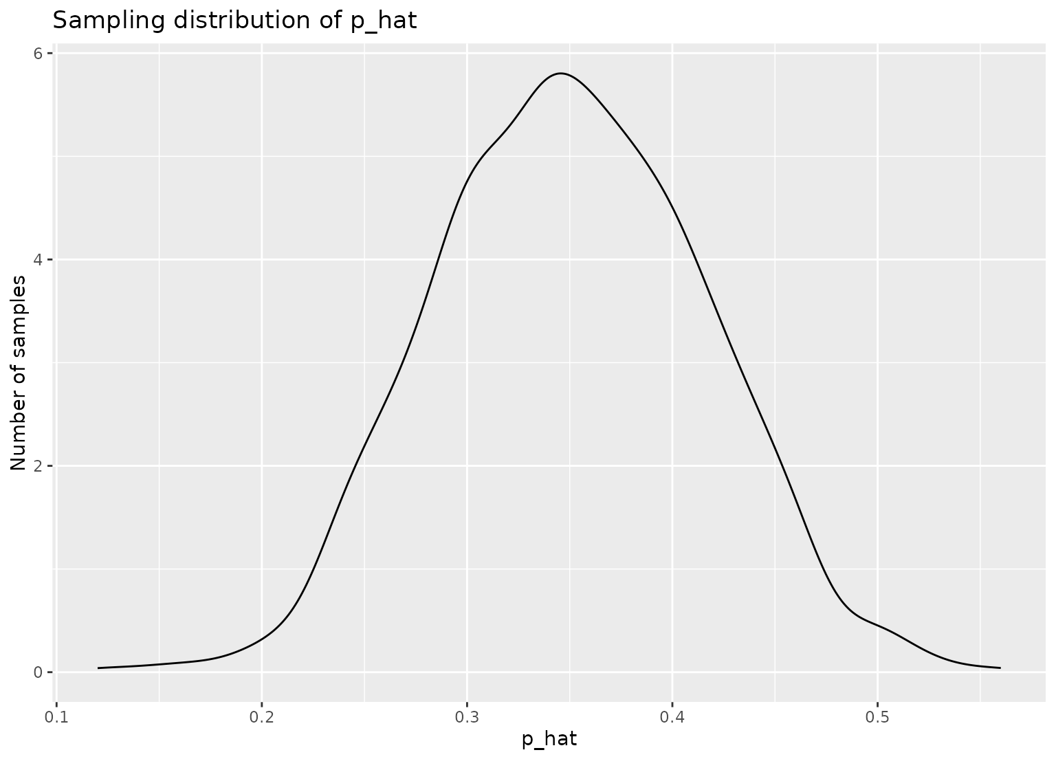
# compute the proportion of respondents with a college
# degree in each replicate
p_hats <- slices %>%
  group_by(replicate) %>%
  summarize(prop_college = mean(college == "degree"))

# plot sampling distribution
ggplot(p_hats, aes(x = prop_college)) +
  geom_density() +
  labs(
    x = "p_hat", y = "Number of samples",
    title = "Sampling distribution of p_hat"
  )


# sampling with probability weights. Note probabilities are automatically
# renormalized to sum to 1
df <- tibble(
  id = 1:5,
  letter = factor(c("a", "b", "c", "d", "e"))
)

rep_slice_sample(df, n = 2, reps = 5, weight_by = c(.5, .4, .3, .2, .1))
#> # A tibble: 10 × 3
#> # Groups:   replicate [5]
#>    replicate    id letter
#>        <int> <int> <fct> 
#>  1         1     1 a     
#>  2         1     2 b     
#>  3         2     1 a     
#>  4         2     4 d     
#>  5         3     1 a     
#>  6         3     3 c     
#>  7         4     2 b     
#>  8         4     1 a     
#>  9         5     1 a     
#> 10         5     5 e